Technical description of main components

In this chapter the mathematical models of components, that are used in ReSiE for the simulation of energy systems, are described. In this context a component is defined as one energy processing part (e.g. a heat pump) of the overall system, while the combination of multiple interconnected components is defined as an energy system. For each component the implemented calculation rules and relevant physical quantities and parameters are described. You can find a detailed description of customizable parameters in thecorresponding chapter.

Note: Not all components described here are implemented in ReSiE yet but all will be included in upcoming versions! Currently, only simplified component models are integrated. Also, the descriptions are not yet completed and may change later.

Convention

Symbols:

• Scalars are shown in italic letters (normal math: $T \ t$)
• Vectors or time series in bold and italic letters (boldsymbol: $\boldsymbol{T \ t}$)
• Matrices are bold and non-italic (textbf: $\textbf{T t}$)

Components:

• Energy flows into a component are positive, energy flows out of a component are negative
• Components are single units like a heat pump, a buffer tank, a battery or a photovoltaic power plant while energy systems are interconnected components

Heat pump (HP)

General description of HP

As heat pumps, electrically driven variable-speed and on-off compressor heat pumps can be integrated into the simulation model of ReSiE. Their general system chart with the denotation of the in- and outputs is shown in the figure below. In general, a gaseous refrigerant is compressed by the compressor requiring electrical energy, resulting in a high temperature of the refrigerant. The refrigerant is then condensed in the condenser and it releases the energy to the condenser liquid at a high temperature level. After that, the refrigerant is expanded and completely liquefied in the expansion valve. In the following evaporator, the refrigerant is then evaporated at a low temperature level with the help of a low-temperature heat source, after which it is fed back into the compressor.

The energy balance at the heat pump is built up from the incoming electricity $P_{el,HP}$, the incoming heat at a low temperature level $T_{HP,source,in}$ and the outgoing heat flow at a higher temperature level $T_{HP,sink,out}$.

The energy balance of the heat pump model is shown in the following figure:

Using the electrical power $P_{el,HP, supply}$, reduced by the losses of the power electronics $P_{el,HP, loss}$, an energy flow $\dot{Q}_{HP,in}$ with temperature $T_{HP,source,in}$ is transformed to the energy flow $\dot{Q}_{HP,out}$ with temperature $T_{HP,sink,out}$. The efficiency of the heat pump is defined by the coefficient of performance (COP). The COP determines the electrical power $P_{el,HP}$ required to raise the temperature of a mass flow from the lower temperature level $T_{HP,source,in}$ to $T_{HP,sink,out}$:

$$COP_{HP} = \frac{\dot{Q}_{HP,out}}{P_{el,HP}} \quad \leq \quad COP_{Carnot} = \frac{T_{HP,sink,out}[K]}{T_{HP,sink,out}-T_{HP,source,in} }$$

$$COP_{HP} = \eta_{Carnot} \ COP_{Carnot} \quad \text{with} \quad 0 \leq \eta_{Carnot} \leq 1$$

The COP is always smaller than the maximum possible Carnot coefficient of performance ($COP_{Carnot}$), which is calculated from the condenser outlet and evaporator inlet temperature. The maximum possible COP calculated by Carnot is reduced by the carnot efficiency factor $\eta_{Carnot}$, which is according to [Arpagaus2018]² around 45 % for high temperature heat pumps and around 40 % for conventional heat pumps.

The energy balance (or power balance) of the heat pump can be drawn up on the basis of the latter figure and on the ratio between supplied and dissipated heat power, expressed as the COP:

$$\dot{Q}_{HP,out} = \frac{COP_{HP}}{COP_{HP} -1} \ \dot{Q}_{HP,in} \mathrm{\quad with \quad} \dot{Q}_{HP,out} = \dot{Q}_{HP,in} + P_{HP,el}$$

The power of the heat pump's electric supply, including the losses of the power electronics, is given as:

$$P_{el,HP,supply} = \frac{P_{el,HP}}{\eta_{HP,LE}}$$

Since the temperatures of the heat flows entering and leaving the heat pump, which have not been considered so far, may also be relevant for connected components, the heat outputs can be calculated on the basis of the respective mass flow $\dot{m}$ and the physical properties of the heat transfer medium (specific heat capacity $c_{p}$ and, if applicable, the density $\rho$) by rearranging the following equation:

$$\dot{Q} = \dot{m} \ c_{p} \ (T_{max} - T_{min})$$

As a chiller follows the same principle as a heat pump, the same component can be used to simulate both technologies. The difference is the definition of the efficiency, as for a chiller the useful energy is not $\dot{Q}_{HP,out}$ but $\dot{Q}_{HP,in}$. This leads to the definition of the energy efficiency ratio (EER) for chillers as

$$EER = \frac{\dot{Q}_{HP,in}}{P_{el,HP}} = \frac{\dot{Q}_{HP,out} - P_{el,HP}}{P_{el,HP}} = COP - 1$$

As shown, the COP can be transferred to the EER. In the following, the description is made for heat pumps. The only adaption that has to be done for chillers is the change of the useful energy. Also, the efficiency function needs to be changed to EER ($T_{HP,source,in}$, $T_{HP,sink,out}$) (if used) and for nonlinear part load efficiency the useful energy $\dot{Q}_{HP,in}$ is assumed to be the linear reference energy instead of $\dot{Q}_{HP,out}$ as for heating mode.

Modelling approaches for HP: Overview

According to [Blervaque2015]¹, four different categories are described in the literature when it comes to the simulation of heat pumps:

• quasi-static empirical models: equation-fit models based on discretized manufacturer or certification data fitted to polynomials, used for example in EnergyPlus or TRNSYS
• dynamic empirical models: equation-fit models extended by continuous transient effects
• detailed physical models: thermodynamic approach based on dynamic and refrigerant flow modelling, many parameters required
• simplified physical models or parameter-estimation models: based on physical model, but with less input parameter needed due to internal assumptions

For the simulation of energy systems in an early design phase, for which QuaSi is intended, only quasi-static or dynamic empirical models can be considered due to the lack of detailed information about the technical components used and the computational effort required for physical models. Therefore, an empirical model based on manufacturer data or certification process data is implemented in ReSiE.

There are several aspects to be considered when simulating a heat pump based on equation-fitting, which will be briefly described in the following:

The COP of a heat pump, representing the efficiency in a current timestep, depends highly on the temperature of the source and the requested temperature of the heat demand. Generally speaking, the efficiency and thus the COP decreases with larger temperature differences between source and sink.

Additionally, the maximum thermal power of the heat pump is not constant for different operation temperatures. The available thermal power is decreasing with lower source temperature, an effect that mainly occurs in heat pumps with air as the source medium. The rated power given for a specific heat pump is only valid for a specified combination of sink and source temperature. The specification for the declaration of the rated power is described in DIN EN 14511³.

Furthermore, the efficiency and therefor the COP is changing in part load operation. In the past, mostly on-off heat pump where used, regulating the total power output in a given time span by alternating the current state between on and off. This causes efficiency losses mostly due to thermal capacity effects and initial compression power needed at each start, or rather the compression losses at each shutdown. [Socal2021]¹¹ In the last years, modulating heat pumps are more common, using a frequency inverter at the electrical power input to adjust the speed of the compression motor and therefor affecting the thermal power output. Interestingly, this method leads to an efficiency increase in part load operation with a peak in efficiency at around 30 to 60 % of the nominal power output. In the literature, many research groups have investigated this effect, compare for example to Bettanini2003⁴, Toffanin2019⁵, Torregrosa-Jaime2008⁶, Fuentes2019⁷, Blervaque2015¹ or Fahlen2012⁸.

When heat pumps with air as source medium are used, the losses due to icing effects need to be considered as well.

For a most realistic representation, all four discussed effects need to be considered - temperature-dependent COP, temperature-dependent power, part-load-dependent COP and icing losses. The calculation of these dependencies will be described below.

Modelling approaches for HP: Detail

Temperature-dependent COP

The temperature-dependent COP can be calculated from different methods:

• using the $COP_{Carnot}$ with the carnot efficiency factor $\eta_{Carnot}$ as explained above (easy, simple and fast, but unreal high efficiency with small temperature differences of source and sink)
• looking up the COP in a look-up table in dependence of the condenser outlet and the evaporator inlet temperature (for computational efficiency, lookup-tables are fitted to polynomials in pre-processing)
• COP calculated as fraction of temperature-dependent electrical and thermal power, gained from generally developed polynomials. Here, the temperature-depended variation of the maximal power output of the heat pump can be directly taken into account.

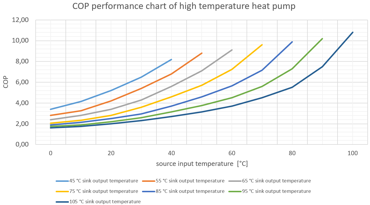
As example for a lookup-table COP (second bulletpoint above), the following figure from Steinacker2022³¹ shows a map of a high-temperature heat pump as a set of curves, depending on the evaporator inlet and condenser outlet temperature. In three dimensions, this figure would result in a surface that can be parameterized with a three-dimensional spline interpolation algorithm.

Maximum thermal and electrical power

In order to address a change in maximum power output or input of the heat pump at different operating temperatures, two different approaches can be used.

The more complex but also more accurate approach is the use of polynomial fits of temperature-dependent thermal and electrical power. These polynomials depend on the condenser outlet and the evaporator inlet temperature and they need to be calculated from manufacturer data or from measurements.

In order to address the early planning stage, general, market-averaged polynomials need to be created, representing an average heat pump. Additionally, one specific heat pump model can be used if the the required data is available.

ToDo: Add method of calculating market-averaged polynomials!

Biquadratic polynomials according to TRNSYS Type 401 $$\dot{Q}_{HP,max} = c_{q1} + c_{q2} \ \bar{T}_{HP,source,in} + c_{q3} \ \bar{T}_{HP,sink,out} + c_{q4} \ \bar{T}_{HP,source,in} \ \bar{T}_{HP,sink,out} + \cdot \cdot \cdot \\ \ c_{q5} \ \bar{T}_{HP,source,in}^2 + c_{q6} \ \bar{T}_{HP,sink,out}^2$$

$$P_{el,HP,max} = c_{p1} + c_{p2} \ \bar{T}_{HP,source,in} + c_{p3} \ \bar{T}_{HP,sink,out} + c_{p4} \ \bar{T}_{HP,source,in} \ \bar{T}_{HP,sink,out} + \cdot \cdot \cdot \\ \ c_{p5} \ \bar{T}_{HP,source,in}^2 + c_{p6} \ \bar{T}_{HP,sink,out}^2$$ where all temperatures have to be normed according to $$\bar{T} = \frac{T \ [°C]}{273.15} + 1$$

If both the thermal output and electrical input power are given as a temperature-dependent polynomial, the temperature-dependent COP (see previous section) can be directly calculated from these polynomials.

The second method to adjust the electrical and thermal energy would be a linear gradient that adjust the rated power in dependency of one temperature. Checking the available data of many different heat pumps from Stiebel-Eltron⁹, a simplified correlation can be observed:

• the thermal power is dependent on the source temperature, but independent on the sink temperature (the lower the source temperature the lower is the heating power)
• the electrical power is dependent on the sink temperature, but independent on the source temperature (the higher the sink temperature the higher is the electrical power consumption)

This gives the possibility to linearly adjust the available thermal power with the change of the source temperature and the electrical power demand with the change of the temperature of the sink. Which power needs to be adjusted depends on the choice of the control strategy - thermally or electrically controlled. The gradients of the power de- or increase with a change of the temperature, $f_{HP,\dot{Q} reduction}$ and $f_{HP,P_{el} reduction}$, needs to be specified. Both factors can have a value of, for example, 0.02, which means a change of 2 % of the rated power per Kelvin of temperature shift with respect to the rated temperatures. The two factors are defined as follows:

$$\dot{Q}_{HP,out,temp. \ dependent} = \dot{Q}_{HP,out,rated} (1 + f_{HP,\dot{Q} reduction} \ (T_{HP,source,in,current} - T_{HP,source,in,rated}))$$ $$P_{el,HP,temp. \ dependent} = P_{el,HP,rated} (1 + f_{HP,P_{el} reduction} \ (T_{HP,sink,out,current} - T_{HP,sink,out,rated}))$$

With this method, the actual temperature-dependent relation of thermal and electrical power need to be determined using the temperature-dependent COP described earlier.

Part load efficiency

The COP of the modeled heat pump depends not only on the temperatures of the sink and the source but also on the current part load ratio (PLR). The COP can be corrected using a part load factor (PLF) that is dependent of the PLR. The definition of the PLR and the PLF is given below:

PLR (part load ratio) $= \frac{\text{power (el. or th.) of demand or availability in current timestep}}{\text{maximum power (el. or th.) of heat pump at current temperatures}}$

PLF (part load factor = adjustment factor for COP): $COP_{part-load} = COP_{full-load} * PLF(PLR)$

The literature provides different examples for the correlation of the COP to the PLR (see section "Overview" for literature examples). This relation is non-linear as shown for example in the following figure given the part-load-dependent COP of an inverter-driven ENRGI-Heatpump at different temperature levels (Source: Enrgi¹⁰).

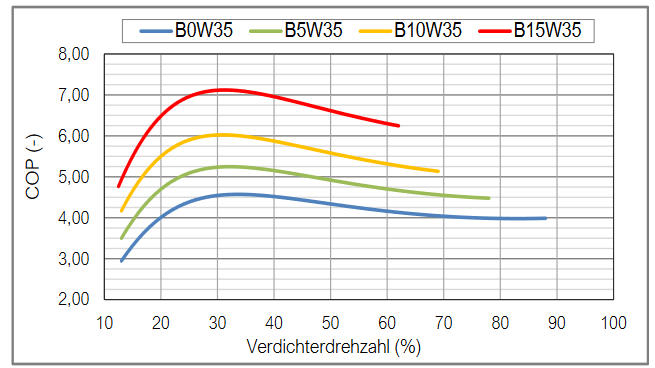
The part-load behavior depends also on the type of the heat pump (on-off or inverter heat pump), as shown for example in Bettanini2003⁴ or in Socal2021¹¹. For illustration, the following figure is taken from the latter reference to demonstrate the different part load factors of the COP (y-axis) at different part load ratios for different heat pump technologies:

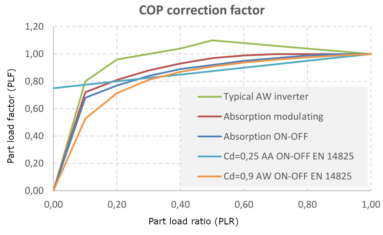
Taking the correction factor curve from the figure above for inverter heat pumps, the maximum part load factor is reached at 50 % part load with an increase of the COP by about 10%. Contrary, in Toffanin2019⁵, the part load factor is assumed to be much higher, reaching its maximum at 25 % part load ratio with a part load factor of 2.1 (efficiency increase of 110 %). These discrepancies illustrate the wide range of literature data and the difficulty in finding a general part load curve. In Lachance2011[Lachance2021^], several part load curves are compared.

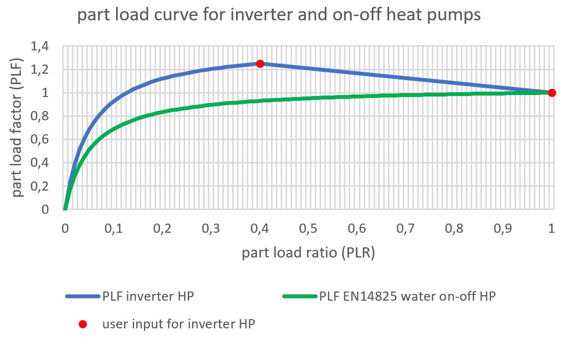
The figure above shows also the difference of the part load factor comparing on-off and inverter heat pumps as well as the defined on-off losses in DIN EN 14825 for the calculation of the seasonal coefficient of performance (SCOP).

As described in the section "General description of HP", the COP is defined as the ratio of the heat output $\dot{Q}_{HP,out}$ and the electrical input power $P_{el,HP}$. The shown curves for the part load factor affects only the ratio of heat output to electrical input power and there is no information available on the actual change of the two dimensions. Therefore, the heat output of the heat pump itself is assumed to be linear in part load operation between $\dot{Q}_{HP,out,min}$ at $PLF_{HP,min}$ and $\dot{Q}_{HP,out,max}$ at PLR = 1.0 as shown in the figure below. This leads to a non-linear relation of the power input to the part load ratio that was found more realistic as for inverter heat pumps, the observed efficiency change is mostly due to an efficiency change of the frequency converter and motor of the compressor. (QUELLE ToDo)

It is also important to note, that the typical PLF-curve for inverter-driven heat pumps is not invertible and can therefore not be used directly to calculate the PLR from PLF. Although, this needed for an operation strategy that uses limited availability or demand of the electrical or thermal power. To handle this problem, the PLF-curve is not used directly:

During preprocessing, the given curve of the PLF in dependence of the PLR (see orange curve in figure below as example) is discretized. Then, the electrical input power (yellow curve) is calculated at each discretization using the assumption of a linear thermal power output (grey curve) in part load operation. As the relation of the power input to the thermal power output is defined by the COP that is changing in every timestep, any COP can be chosen for this initial calculation during the preprocessing. For this example, a COP of 4 is chosen. This process results in two value tables for the electrical input power and the thermal output power. The latter one is, according to the assumption made above, a straight line as shown in the figure.

Both value tables are then normalized to their maximum value as shown in the next figure. The thermal power input although can not be precalculated as it depends on the absolute difference of thermal output and electrical input power.

In every timestep, the two precomputed and normalized value tables of the thermal output and electrical input power are scaled up to the current maximum power, limited by the heat pump current full-load operation state. There, the actual COP at the current timestep is represented in the ration of both values. The two scaled value tables can then be used to determine the actual PLF that is necessary to cover the current demand or to limit the operation state due to the limited available electrical power (interpolation on value table with known power, or interpolation in preprocessing). For the thermal output power, this is trivial as the ratio of the maximum thermal power output to the thermal power demand is equal to the PLF. To calculate the PLF for the thermal input power, if this is a limited source according to the operational strategy, the two scaled value tables need to be subtracted from each other to get a third table:

$$\dot{Q}_{HP,in}(PLF) = \dot{Q}_{HP,out}(PLF) - P_{el,HP,in}(PLF)$$

This third value table, generated in each timestep, can then be used to determine the maximum possible PLF according to the available thermal input power from a limited thermal power source.

All three PLF (from thermal input and output as well as electrical input power) are then compared and the smallest one is chosen as operating state in the current timestep. If this value is smaller than the minimal allowed PLF of the heat pump $PLF_{HP,min}$, the heat pump will not be in operation in the current timestep.

This method avoids the need to invert polynomial functions at each timestep and is computationally more efficient.

The definition of the part load factor curve is user-defined and differentiated into inverter and on-off heat pumps. The part load factor curve for inverter-driven heat pumps is based on Blervaque2015¹ and Filliard2009¹². There, the curve is defined in two separate sections. The section below the point of maximum efficiency is a function according to the part load factor calculation in DIN EN 14825 for water-based on-off heatpumps, differing from the cited paper but according to Fuentes2019⁷. The section above the point of the maximum efficiency is approximated as straight curve. The definition of these curve can be done entering the cc-coefficient and the coordinates of the two points highlighted in the figure below. Here, cc is chosen as 0.95 and $a$ is used to stretch the curve to meet the intersection point with the straight line.

This results in the following equation to calculate the part load factor for inverter-driven heat pumps, defined by the coefficients cc and a according to DIN EN 14825, the point of maximum efficiency at ($PLR_{max}$/$PLF_{max}$) and the PLR_1 at PLF = 1:

$$PLF(PLR) = \begin{cases} a \ \frac{PLR}{cc \ PLR + (1 - cc)} & \text{ for } PLR < PLR_{max} \\ \frac{PLF_1 - PLF_{max}}{1-PLR_{max}} \ ( PLR - PLR_{max} ) + PLF_{max} & \text{ for } PLR >= PLR_{max} \end{cases} \\ \text{ with } a = \frac{PLF_{max}}{PLR_{max}} \left ( cc \ (PLR_{max}-1)+1 \right )$$

For on-off heat pumps, $a$ is set to 1 and the domain of the first equation above is set to the whole range of the PLR.

Icing-losses of heat pumps with air as source medium

To account for icing losses of heat pumps with air as source medium, the approach presented in TRNSYS Type 401 is used¹⁵. When considering icing-losses, make sure that icing losses are not already included in the polynomials for thermal and electrical power!

For the calculation of icing losses, five coefficients are needed: $c_{HP,ice,A}$, $c_{HP,ice,B}$, $c_{HP,ice,C}$, $c_{HP,ice,D}$ and $c_{HP,ice,E}$. According to the Type 401, icing losses are calculated using a superposition of a gaussian curve with its maximum between 0 °C and 5 °C representing the maximum likelihood of frost within the heat pump (high absolute humidity) and a linear curve, representing the higher sensible energy effort to heat-up the components of the heat pump for defrosting. Exemplary curves are shown in the following figure (linear, gauss and superposition):

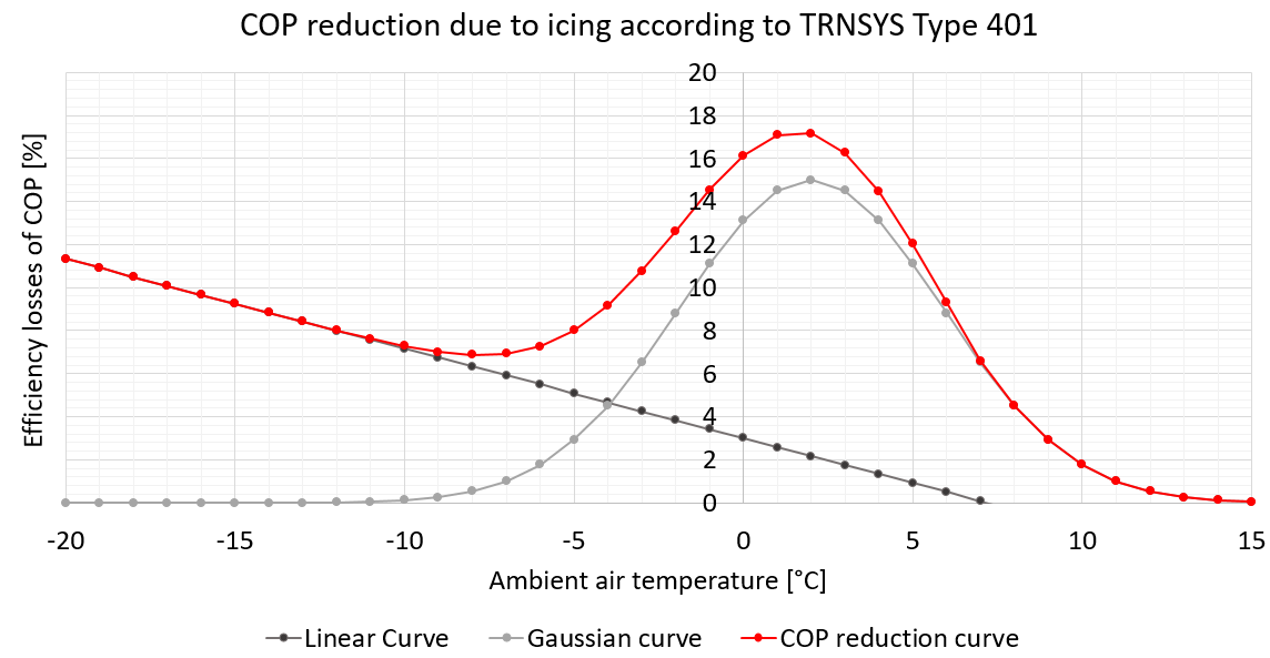
The exemplary coefficients for the curves in the figure above are $c_{HP,ice,A} = 3$, $c_{HP,ice,B} = -0.42$, $c_{HP,ice,C}=15$, $c_{HP,ice,D}=2$, $c_{HP,ice,E}=30$.

The resulting superposition, which represents the percentage loss of the COP due to icing as a function of ambient temperature, is expressed by the following formula, where the coefficients are reduced to the last letter for better readability: $$\Delta COP_{ice,loss} = \begin{cases} A + B \ T_{HP,source,in} + C \ exp^{-\frac{(T_{HP,source,in}-D)^2}{E}} &\text{for } A + B \ T_{HP,source,in} > 0\ \\[5pt] C \ exp^{-\frac{(T_{HP,source,in}-D)^2}{E}} &\text{for } A + B \ T_{HP,source,in} \leq 0\ \\ \end{cases} \\ $$

$\Delta COP_{ice,loss}$ can then be used to reduce the COP for icing losses:

$$COP_{ice,corrected} = COP \ (1-\Delta COP_{ice,loss})$$

According to the results found in Wei2021¹⁴, it is assumed that the decrease of the COP due to icing losses will only increase the power input of the heat pump. It will not affect the thermal power output.

Steps to perform in the simulation model of the heat pump

The calculation is based on TRNSYS Type 401¹⁵ that is almost similar to Type 204¹⁶ (Type 204 provides an english documentation). The cycling losses of the heat pump in both TRNSYS models are calculated using an exponential function to describe the thermal capacity effects during heat-up and cool-down. Here, these cycling losses will only be used during start and stop of the heat pump - actual cycling losses from on-off heatpumps will be considered separately in the process to allow the consideration of modulating heat pumps as well.

There are two different possibilities in calculating the full load power of the heat pump in dependence of $T_{HP,sink,out}$ and $T_{HP,source,in}$. An overview of the simulation steps and the required inputs are given in the following figure. A detailed description of the process shown in the figure is given below. Each of the main steps is described in more detail in the previous chapter.

Steps to calculate the electrical and thermal energy in- and outputs of HP using a polynomial fit of the thermal and electrical power (compare to left side of figure above):

• using polynomial fits to calculate stationary thermal in- and output and electrical full-load power at given temperatures of $T_{HP,sink,out}$ and $T_{HP,source,in}$ for given nominal thermal power
  • differing source and sink medium:
    • air-water
    • water-water
    • sole-water
  • differing temperature range:
    • normal heat pump
    • high-temperature heat pump
  • polynomial fits have to be normalized to rated power at specified temperatures! Rated power has to be related always to the same temperature lift according to DIN EN 14511 --> different fits for normal (B10/W35, W10/W35, A10/W35) and high temperature (B35/W85, W35/W85) heat pumps
• reduce thermal power output due to transient capacity effects during start-up as average over current timestep and calculate COP$_{transient}$ at full load with calculated thermal and electrical power
• may adjust COP$_{transient}$ by icing losses for air-water and air-air heat pumps; calculate COP$_{transient,ice}$, recalculate electrical input power
• get demand/availability of thermal or electrical energy (mind $\eta_{HP,PE}$!), differing if thermal and/or electric energy related operation strategy is chosen
• calculate smallest non-linear part-load ratio (PLR) with current demand and temperature-dependent, transient full-load power and precalculated value tables from PLF-curve, in dependency of heat pump type (inverter, on-off)
• calculate part-load thermal and electrical energy, recalculate COP$_{transient,ice,partload}$

If universal data table or the Carnot-COP reduced by an efficiency factor should be used instead of the more accurate model described above, a different calculation approach is needed (compare right side in the figure above):

• Get power at current temperatures
  • using nominal power without a temperature-dependency or
  • using polynomial fits to calculate stationary thermal or electrical full-load power at given temperatures of $T_{HP,sink,out}$ and $T_{HP,source,in}$, depending on control strategy (see above)
• get stationary full-load COP at given temperatures of $T_{HP,sink,out}$ and $T_{HP,source,in}$ either from
  • COP data table (fitted to polynomials in pre-calculation) or
  • Carnot-COP reduced by an efficiency factor
• determine the unknown, non-controlled full load power (electrical or thermal) with known, controlled power and COP
• continue with transient capacity effects as described above

Contrary to the TRNSYS Type 401, the mass flow here is variable and not constant within two time steps, therefore the $T_{HP,sink,out}$ and $\dot{Q}_{HP,sink,out}$ can be calculated directly without the need of iteration as implemented in Type 401. Here, the $T_{HP,sink,out}$ is a fixed, user-specified value in the presented simplified model.

The polynomials describing the temperature-depended thermal and electrical power of the heat pump need to be normalized to the power consumption at the rated operation point in order to be able to auto-scale the size in parameter variation studies. Therefore, the following steps are necessary:

• fit data to polynomial for thermal and electrical energy
• calculate power at specified nominal temperatures with generated fitted polynomial
• normalize polynomial to calculated rated power at specific temperature using a fraction_factor

Inputs und Outputs of the Heat Pump:

Symbol	Description	Unit
$\dot{Q}_{HP,in}$	heat flow supplied to the HP (heat source)	[W]
$\dot{Q}_{HP,out}$	heat flow leaving the HP (heat sink)	[W]
$P_{el,HP}$	electric power demand of the HP	[W]
$P_{el,HP,supply}$	electric power demand of the HP incl. losses of the power electronics	[W]
$T_{HP,sink,in}$	condenser inlet temperature - not used	[°C]
$T_{HP,sink,out}$	condenser outlet temperature	[°C]
$T_{HP,source,in}$	evaporator inlet temperature	[°C]
$T_{HP,source,out}$	evaporator outlet temperature - not used	[°C]

Parameter of the Heat Pump:

Symbol	Description	Unit
$\dot{Q}_{HP,rated}$	rated thermal energy output of heat pump at specified conditions	[W]
$\dot{Q}_{HP,max}(T_{HP,sink,out}, T_{HP,source,in})$	(normalized) polynomial of maximum full load thermal heat output at given temperatures	[W]
$P_{el,HP,max}(T_{HP,sink,out}, T_{HP,source,in})$	(normalized) polynomial of maximum full load electrical power output at given temperatures	[W]
or
$f_{HP,\dot{Q} reduction}$	linear reduction factor for nominal full load thermal output power with respect to $T_{HP,source,in}$	[%/°C]
$f_{HP,P_{el} reduction}$	linear reduction factor for nominal full load electrical input power with respect to $T_{HP,sink,out}$	[%/°C]
$COP_{HP}(T_{HP,sink,out}, T_{HP,source,in})$	coefficient of performance (COP) of the heat pump depending on $T_{HP,sink,out}$ and $T_{HP,source,in}$	[-]
$\eta_{Carnot}$	efficiency factor of heat pump, reduces the Carnot-COP	[-]
and
$PL_{HP,min}$	minimum possible part load of the heat pump	[%]
$PLR_{HP,max}$	part load ratio at point of maximum efficiency (inverter only)	[-]
$PLF_{HP,max}$	part load factor at point of maximum efficiency (inverter only)	[-]
$PLF_{HP,PLR=1}$	part load factor at part load ratio = 1 (inverter only)	[-]
$cc_{HP}$	coefficient for part load curve according to DIN EN 14825	[-]
$c_{HP,ice,A} \ : \ c_{HP,ice,E}$	five coefficients for curve with icing losses according to TRNSYS Type 401 (air heat pump only)	[-]
$\eta_{HP,PE}$	efficiency of power electronics of heat pump	[-]
$MOT_{HP}$	minimum operating time of heat pump	[min]
$SUT_{HP}$	start-up time of the HP until full heat supply (linear curve)	[min]
$CDT_{HP}$	cool-down time of the HP from full heat supply to ambient (linear curve)	[min]

State Variables of Heat Pump:

Symbol	Description	Unit
$x_{HP}$	current operating state (on, off, part load)	[%]

Hydrogen Electrolyser (HEL)

The hydrogen electrolyser uses electrical energy to split water into its components hydrogen ($H_2$) and oxygen ($O_2$) as shown in the following reaction equation:

$$2 \ H_2O \rightarrow 2 \ H_2 + O_2$$

If the electrical energy is provided by renewable energies, the resulting hydrogen is labeled as "green hydrogen" and can be used to decarbonize the mobility or industrial sector or fed into the natural gas grid. The waste heat generated in the process can be used directly by feeding it into a heat network or via an intermediate heat pump. For flexible operation, it is possible to discharge the waste heat to the environment using a chiller. The use of waste heat is an important factor for the overall efficiency of the electrolyser.

The general energy and mass flow in the electrolyser as well as the losses considered in the model can be seen in the following figure.

The relationship between supplied hydrogen of the electrolysis (energy ($\dot{E}_{HEL,H_2}$) or mass flow ($\dot{m}_{HEL,H_2}$)) and the consumption of electrical energy ($P_{el,HEL}$) is given in the following equation, where $e_{H_2}$ can be either the net or the gross calorific value of the hydrogen: $$\begin{align} \dot{E}_{HEL,H_2}= P_{el,HEL} \enspace \eta_{HEL,H_2} \end{align}$$

$$\begin{equation} \dot{m}_{HEL,H_2} = \frac{\dot{E}_{HEL,H_2}}{e_{H_2}} \end{equation}$$

Due to the purification losses of the hydrogen caused by the reduction of oxygen molecules contained in the hydrogen gas in the catalyst, depending on the electrolysis technology, the actually obtained hydrogen energy or mass flow is reduced by the proportion of the hydrogen losses $\eta_{H_2 \ purification}$ to the energy or mass flows, supplemented with index $out$: $$\dot{E}_{HEL,H_2,out}= (1-\eta_{H_2 \ purification}) \ \dot{E}_{HEL,H_2}$$

$$\dot{m}_{HEL,H_2,out} = (1-\eta_{H_2 \ purification}) \ \dot{m}_{HEL,H_2}$$

Conversely, by rearranging and substituting the previous equations from a required hydrogen mass flow, the electrical power consumption can be calculated as follows: $$P_{el,HEL} = \frac{\dot{m}_{HEL,H_2,out} \ e_{H_2}}{\eta_{HEL,H_2} \ (1 - \eta_{H_2 \ purification})}$$

The usable waste heat from the electrolysis process $\dot{Q}_{HEL,waste heat}$ is determined, depending on the available information, as $$\dot{Q}_{HEL,waste heat} = \eta_{HEL,heat} \enspace (1-\eta_{HEL,H_2}) \enspace P_{el,HEL} = \frac{(1 - \eta_{HEL,H_2}) \ \eta_{HEL,heat} } { (1 - \eta_{H_2 \ purification}) \ \eta_{HEL,H_2} } \ \dot{E}_{HEL,H_2,out}$$

With an increase of operation time, the efficiency in hydrogen production of the stacks of electrolysers is decreasing while the efficiency of heat production is increased. This is due to degradation effects in the stacks. This effect of aging of the stack cells can be expressed by an correction factor for each the hydrogen ($\delta_{HEL,H_2} < 0$) and the heat ($\delta_{HEL,heat}$ > 0) related efficiency. These correction factors are given in the change of percentage points per 10.000 full load hours (FLH), where the full load hours are determined by dividing the total hydrogen produced by the nominal hydrogen output of the electrolyser. The efficiencies of hydrogen and heat production are therefore corrected in every timestep using the nominal efficiency at the point of the beginning of life of the electrolyser, the correction factors and the passed FLH.

$$\eta_{HEL,H_2} = \eta_{HEL,H_2,start} + \left ( \frac{\delta_{HEL,H_2}}{100} \ {\frac{FLH}{10.000}} \right )$$ $$\eta_{HEL,heat} = \eta_{HEL,heat,start} + \left ( \frac{\delta_{HEL,heat}}{100} \ {\frac{FLH}{1.000}} \right )$$ $$\text{with } FLH = \frac{\text{total hydrogen produced since start [kg]}}{\text{nominal hydrogen production [kg]}}$$

Keep in mind: Test if sum of efficiencies will reach values > 1 or if one efficiency falls below zero for the given maximum changing intervale of the stacks (ToDo)

With a known mass flow $\dot{m}_{HP,cool}$ and the specific heat capacity of the heat transfer medium of the heat recovery $c_{p,cool}$ as well as a known inlet temperature $T_{HEL,cool,in}$, the outlet temperature of the heat transfer medium from the cooling circuit $T_{HEL,cool,out}$ can be determined by rearranging the following equation: $$\dot{Q}_{HEL,waste heat} = \dot{m}_{HP,cool} \enspace c_{p,cool} \enspace (T_{HEL,hot,out} - T_{HEL,cool,in})$$

The heat loss $\dot{Q}_{HEL,loss}$, which cannot be used and is dissipated to the environment via heat transport mechanisms, is calculated as follows

$$\dot{Q}_{HEL,loss} = P_{el,HEL} - \dot{Q}_{HEL,waste heat} - \dot{E}_{HEL,H_2} \\ = P_{el,HEL} \ (1 - \eta_{HEL,heat} + \eta_{HEL,heat} \ \eta_{HEL,H_2} - \eta_{HEL,H_2})$$

The actual needed power supply of the electrolyser $P_{el,HEL,supply}$ increases by losses in the power electronics and results from the electrical reference power $P_{el,HEL}$ and the losses in the power electronics $\eta_{HEL,PE}$ to $$P_{el,HEL,supply} = \frac{P_{el,HEL}}{\eta_{HEL,PE}}$$

Since the oxygen produced during the electrolysis process can also be utilized economically under certain circumstances, the resulting oxygen mass flow $\dot{m}_{HEL,O_2,out}$ is determined from the stoichiometric ratio of the reaction equation of the water splitting described at the beginning:

$$\dot{m}_{HEL,O_2,out} = v_{O_2,H_2} \enspace \dot{m}_{HEL,H_2}$$ $$\text{with} \quad v_{O_2,H_2} = \frac{atomic \ mass \ O_2}{atomic \ mass \ 2 \ H_2} = \frac{2 * 15,9990 \ u}{2*2*1,0008 \ u} = 7,9386$$

The required mass flow of water $\dot{m}_{HEL,H_2O,in}$ can be determined from the supplied masses of hydrogen and oxygen and the purification losses in the water treatment unit, characterized by the fraction of purification losses $\eta_{H_2O \ treatment}$. $$\dot{m}_{HEL,H_2O,in} = \frac{\dot{m}_{HEL,H_2} + \dot{m}_{HEL,O_2,out}}{1- \eta_{H_2O \ treatment}}$$

Assumption: The electrolyser is only operated between minimum 0 % and maximum 100 % load. A specification of power above nominal power, which frequently occurs in practice, is not supported.

Inputs and Outputs of the Electrolyser:

Symbol	Description	Unit
$P_{el,HEL}$	electrical power requirement of the electrolyser	[W]
$P_{el,HEL,supply}$	electrical power requirement of the electrolyser incl. losses of power electronics	[W]
$\dot{m}_{HEL,H_2O,in}$	water mass flow fed to the electrolyser	[kg/h]
$\dot{m}_{HEL,O_2,out}$	oxygen mass flow delivered by the electrolyser	[kg/h]
$\dot{m}_{HEL,H_2}$	hydrogen mass flow produced by the electrolyser (before $H_2$-cleaning losses)	[kg/h]
$\dot{m}_{HEL,H_2,out}$	hydrogen mass flow provided by the electrolyser (after $H_2$-cleaning losses)	[kg/h]
$\dot{E}_{HEL,H_2}$	hydrogen energy flow discharged from the electrolyser (before $H_2$-cleaning losses)	[W]
$\dot{E}_{HEL,H_2,out}$	hydrogen energy flow provided by the electrolyser $after (H_2$-cleaning losses)	[W]
$T_{HEL,cooling,in}$	cooling fluid inlet temperature of electrolyser	[°C]
$T_{HEL,cooling,out}$	cooling fluid outlet temperature of electrolyser	[°C]
$\dot{Q}_{HEL,waste heat}$	waste heat provided by the electrolyser	[W]
$\dot{Q}_{HEL,loss}$	thermal losses in electrolyser (unused waste heat))	[W]

Parameter of the Electrolyser:

Symbol	Description	Unit
$P_{el,HEL,rated}$	electric power consumption of the electrolyser under full load (operating state 100 %)	[W]
$\eta_{HEL,H_2,start}(x_{HEL},P_{el,HEL,rated})$	efficiency of hydrogen production of the electrolyser ($\dot{E}_{HEL,H_2,out}$ related to $P_{el,HEL}$ as a function of operating state, plant size and plant type at the beginning of live)	[-]
$\eta_{HEL,heat,start}$	efficiency of the usable heat extraction of the electrolyser (related to $1-\eta_{HEL,H_2}$ at the beginning of live)	[-]
$\delta_{HEL,H_2}$	linear decrease of efficiency of hydrogen production due to degradation per 10.000 full load hours, typically < 0	$\left [ \frac{\%-points}{\text{10.000 full load hours}}\right ]$
$\delta_{HEL,heat}$	linear increase of efficiency of heat production due to degradation per 10.000 full load hours, typically > 0	$\left [ \frac{\%-points}{\text{10.000 full load hours}}\right ]$
$\eta_{HEL,LE}$	efficiency of the power electronics of the electrolyser	[-]
$PL_{HEL,min}$	minimum allowed partial load of the electrolyser	[-]
$MOT_{HEL}$	minimum operating time of the electrolyser	[min]
$SUT_{HEL}$	start-up time of the electrolyser until full heat supply (linear curve)	[min]
$CDT_{HEL}$	cool-down time of the electrolyser from full heat supply to ambient (linear curve)	[min]
$e_{H_2}$	mass-dependent energy of hydrogen (net calorific value or gross calorific value)
$v_{O_2,H_2}$	stoichiometric mass-based ratio of oxygen and hydrogen supply during electrolysis	[kg $O_2$ / kg $H_2$]
$\eta_{H_2 \ purification}$	percentage of purification losses in hydrogen purification	[%]
$\eta_{H_2O \ treatment}$	percentage of purification losses in water treatment	[%]
$p_{H_2,HEL}$	pressure of hydrogen supply	[bar]
$p_{O_2,HEL}$	pressure of oxygen supply	[bar]
$T_{HEL,cooling,in,max}$	max. allowed temperature of cooling medium input	[°C]

State variables of the Electrolyser:

Symbol	Description	Unit
$x_{HEL}$	current operating state (on, off, part load)	[%]

Combined heat and power plant (CHPP)

Energy balance on CHPP: $$\dot{E}_{CHPP,gas,in} = P_{el,CHPP,out} + \dot{Q}_{CHPP,out} + \dot{Q}_{CHPP,loss}$$

Calculation of electric power output: $$P_{el,CHPP,out} = \eta_{CHPP,el} \ \dot{E}_{CHPP,gas,in}$$

Calculation of thermal power output: $$\dot{Q}_{CHPP,out} = \eta_{CHPP,thermal} \ \dot{E}_{CHPP,gas,in}$$

Calculation of thermal losses in CHPP: $$\dot{Q}_{CHPP,loss} = (1-\eta_{CHPP,thermal}+\eta_{CHPP,el}) \ \dot{E}_{CHPP,gas,in}$$

Relation of electric and thermal power output: $$P_{el,CHPP,out} = \frac{\eta_{CHPP,el}}{\eta_{CHPP,thermal}} \ \dot{Q}_{CHPP,out} = r_{CHPP,PTH} \ \dot{Q}_{CHPP,out}$$

The part-load dependent efficiency as described in the chapter "general transient effects" can be considered as well.

ToDo: part-load dependent efficiency definition with heat and electricity --> two efficiency curves? One efficiency curve and the second one related to the first one? Part load curve e.g in Urbanucci2019¹⁷

Inputs and Outputs of the CHPP:

Symbol	Description	Unit
$P_{el,CHPP,out}$	electric power output of the CHPP	[W]
$P_{el,CHPP}$	electric power provided by the CHPP	[W]
$\dot{Q}_{CHPP,out}$	thermal power output of the CHPP	[W]
$\dot{E}_{CHPP,gas,in}$	energy demand of the CHPP, natural or green gas (NCV or GCV)	[W]
$\dot{Q}_{CHPP,loss}$	thermal energy losses of the CHPP	[W]

Parameter of the CHPP:

Symbol	Description	Unit
$P_{el,CHPP,rated}$	rated electric power output of the CHPP under full load (operating state 100 %)	[W]
$\dot{Q}_{CHPP,rated}$	rated thermal power output of the CHPP under full load (operating state 100 %)	[W]
$\eta_{CHPP,thermal}(PLR)$	thermal efficiency of CHPP, function of PLR (regarding NCV or GCV, needs to correspond to $\dot{E}_{CHPP,gas,in}$)	[-]
$\eta_{CHPP,el}(PLR)$	electrical efficiency of CHPP, including self-use of electrical energy, function of PLR (regarding NCV or GCV, needs to correspond to $\dot{E}_{CHPP,gas,in}$)	[-]
$PL_{CHPP,min}$	minimum allowed partial load of the CHPP	[-]
$MOT_{CHPP}$	minimum operating time of the CHPP	[min]
$SUT_{CHPP}$	start-up time of the CHPP until full heat supply (linear curve)	[min]
$CDT_{CHPP}$	cool-down time of the CHPP from full heat supply to ambient (linear curve)	[min]

State variables of the CHPP:

Symbol	Description	Unit
$x_{CHPP}$	current operating state of the CHPP (on, off, part load)	[%]

Gas boiler (GB)

Energy balance of gas boiler: $$\dot{Q}_{GB,out} = \dot{E}_{GB,gas,in} - \dot{Q}_{GB,loss} = \eta_{GB}(PLR) \ \dot{E}_{GB,gas,in}$$

Inputs and Outputs of the GB:

Symbol	Description	Unit
$\dot{Q}_{GB,out}$	thermal power output of the GB	[W]
$\dot{E}_{GB,gas,in}$	energy demand of the GB, natural or green gas (NCV or GCV)	[W]
$\dot{Q}_{GB,loss}$	thermal losses of the GB	[W]

Parameter of the GB:

Symbol	Description	Unit
$Q_{GB,rated}$	rated thermal power output of the GB under full load (operating state 100 %)	[W]
$\eta_{GB}(PLR)$	thermal efficiency of gas boiler (regarding NCV or GCV) with respect to the PLR	[-]
$PL_{GB,min}$	minimum allowed partial load of the GB	[-]
$MOT_{GB}$	minimum operating time of the GB	[min]
$SUT_{GB}$	start-up time of the GB until full heat supply (linear curve)	[min]
$CDT_{GB}$	cool-down time of the GB from full heat supply to ambient (linear curve)	[min]

State variables of the GB:

Symbol	Description	Unit
$x_{GB}$	current operating state of the GB (on, off, part load)	[%]

Oil heating (OH)

Energy balance of oil heater: $$\dot{Q}_{OH,out} = \dot{E}_{OH,oil,in} - \dot{Q}_{OH,loss} = \eta_{OH}(PLR) \ \dot{E}_{OH,oil,in}$$

Inputs and Outputs of the OH:

Symbol	Description	Unit
$\dot{Q}_{OH,out}$	thermal power output of the OH	[W]
$\dot{E}_{OH,oil,in}$	energy demand of the OH, fuel oil (NCV or GCV)	[W]
$\dot{Q}_{OH,loss}$	thermal losses of the OH	[W]

Parameter of the OH:

Symbol	Description	Unit
$Q_{OH,rated}$	rated thermal power output of the OH under full load (operating state 100 %)	[W]
$\eta_{OH}(PLR)$	thermal efficiency of oil heater (regarding NCV or GCV) with respect to the PLR	[-]
$PL_{OH,min}$	minimum allowed partial load of the OH	[-]
$MOT_{OH}$	minimum operating time of the OH	[min]
$SUT_{OH}$	start-up time of the OH until full heat supply (linear curve)	[min]
$CDT_{OH}$	cool-down time of the OH from full heat supply to ambient (linear curve)	[min]

State variables of the OH:

Symbol	Description	Unit
$x_{OH}$	current operating state of the OH (on, off, part load)	[%]

Elecric heating rod (ER)

Energy balance of electric heating rod: $$\dot{Q}_{ER,out} = \dot{P}_{ER,el,in} - \dot{Q}_{ER,loss} = \eta_{ER}(PLR) \ \dot{P}_{ER,el,in}$$

Inputs and Outputs of the ER:

Symbol	Description	Unit
$\dot{Q}_{ER,out}$	thermal power output of the ER	[W]
$\dot{P}_{ER,el,in}$	electrical energy demand of the ER	[W]
$\dot{Q}_{ER,loss}$	thermal losses of the ER	[W]

Parameter of the ER:

Symbol	Description	Unit
$Q_{ER,rated}$	rated thermal power output of the ER under full load (operating state 100 %)	[W]
$\eta_{ER}(PLR)$	thermal efficiency of electric heating rod with respect to the PLR	[-]
$PL_{ER,min}$	minimum allowed partial load of the ER	[-]
$MOT_{ER}$	minimum operating time of the ER	[min]
$SUT_{ER}$	start-up time of the ER until full heat supply (linear curve)	[min]
$CDT_{ER}$	cool-down time of the ER from full heat supply to ambient (linear curve)	[min]

State variables of the ER:

Symbol	Description	Unit
$x_{ER}$	current operating state of the ER (on, off, part load)	[%]

Biomass boiler (BB)

Energy balance of biomass boiler: $$\dot{Q}_{BB,out} = \dot{E}_{BB,biomass,in} - \dot{Q}_{BB,loss} = \eta_{BB}(PLR) \ \dot{E}_{BB,biomass,in}$$

Inputs and Outputs of the BB:

Symbol	Description	Unit
$\dot{Q}_{BB,out}$	thermal power output of the BB	[W]
$\dot{E}_{BB,biomass,in}$	energy demand of the BB, biomass (NCV or GCV)	[W]
$\dot{Q}_{BB,loss}$	thermal losses of the BB	[W]

Parameter of the BB:

Symbol	Description	Unit
$Q_{BB,rated}$	rated thermal power output of the BB under full load (operating state 100 %)	[W]
$\eta_{BB}(PLR)$	thermal efficiency of biomass boiler (regarding NCV or GCV, specific fuel and moisture content) with respect to the PLR	[-]
$PL_{BB,min}$	minimum allowed partial load of the BB	[-]
$MOT_{BB}$	minimum operating time of the BB	[min]
$SUT_{BB}$	start-up time of the BB until full heat supply (linear curve)	[min]
$CDT_{BB}$	cool-down time of the BB from full heat supply to ambient (linear curve)	[min]

State variables of the BB:

Symbol	Description	Unit
$x_{BB}$	current operating state of the BB (on, off, part load)	[%]

Heat sources

Soil

• geothermal probes --> see below
• geothermal collector --> see below
• geothermal basket collector --> not included for now
• geothermal trensh collector --> not included for now
• geothermal spiral collector --> not included for now

Geothermal Probes

Overview

Geothermal probes are vertical geothermal heat exchangers with a typical drilling depth of 50 - 150 m. Into the borehole, which usually has a diameter of 150 - 160 mm, pipes are laid. In most cases, two pipes are inserted into the borehole in a U-shape and the borehole is subsequently filled with filling material. The purpose of the filling material is to improve the thermal properties of the heat transfer between the probe tubes and the ground and to give the borehole stability. Geothermal probes serve as heat reservoirs for heat pumps and can also be used conversely as cold reservoirs in summer regeneration mode. In larger systems, several borehole heat exchangers are connected hydraulically in parallel to form fields of geothermal probes. Over longer periods of time, the temperature fields around adjacent probes in a field influence each other. There are several approaches to model geothermal probes. In ReSiE, an approach based on g-functions is chosen. Using the g-functions, temperature responses of the surrounding earth to changes in thermal in- and output power can be calculated, as illustrated in the figure below. This approach eliminates the need to numerically calculate the temperature field of the entire ground at each time step and is therefore computationally efficient. The g-function values are based on analytical mathematical computational equations, which will be discussed in more detail later.

Basic Simplifications

The soil is assumed to be homogeneous with uniform and constant physical properties over time. The properties can be determined, for example, by a thermal response test, or estimated by assumptions of the soil typology with standard values from VDI 4640-1¹⁸. In addition, it is assumed that the heat transport processes in the ground are based exclusively on heat conduction. Convective effects, like ground water flow, are therefore not taken into account. All probes in the probe field are assumed to be identical in geometry and design and are hydraulically connected in parallel, i.e. the same volume flow rate flows through all of them in each time step. The borehole and fluid temperatures of each individual probe are assumed to be the same and the total heat extraction and input rates are divided equally among all probes.

g-function approach

The general g-function approach was introduced by Eskilson.¹⁹ The current temperature at the borehole wall $T_B$ as response to a specific heat extraction or injection $\tilde{q}_{in,out}$ within one timestep can be determined using the following equation:

$$T_B = T_{s,u} + \frac{\tilde{q}_{in,out}}{2\pi\lambda_s} \cdot g(t)\ $$

where $T_{s,u}$ is the undisturbed ground temperature, $\lambda_s$ is the heat conductivity of the soil and $g(t)$ the pre-calculated g-function value at the current simulation time (\t). $\tilde{q}_{in,out}$ can be calculated with the total heat extraction rate for one single probe $\dot{Q}_{in,out}$, which is constant over each time step, and with the probe depth $h_{\text{probe}}$. $\dot{Q}_{in,out}$ is considered to be uniform over the entire depth of the probe.

$$\tilde{q}_{in,out} = \frac{\dot{Q}_{in,out}}{h_{\text{probe}}}\ $$

Since the heat extraction or injection rate varies with each time step, a superposition approach is chosen, which is based on Duhamels theorem.²⁰ The temperature at the borehole wall $T_B$ is calculated by superimposing the temperature responses to past heat pulses:

$$T_B = T_{s,u} + \sum_{i=1}^n \left[ \frac{\tilde{q}_{in,out,i} - \tilde{q}_{in,out,i-1}}{2\pi\lambda_s} \cdot g(t_n - t_{i-1}) \right]\ $$

The undisturbed ground temperature $T_{s,u}$ can be assumed as a constant value averaged over the probe depth. With the assumption of a thermal borehole resistance $R_{B}$ between the borehole wall and the circulating fluid, an average fluid temperature $T_{\text{fl,avg}}$ can be calculated from the borehole temperature. The calculation approach of the thermal borehole resistance will be discussed in more detail later.

$$T_{\text{fl,avg}} = T_B + \tilde{q}_{in,out} \cdot R_B$$

Since a uniform borehole wall temperature over the entire probe depth is assumed, a depth-averaged fluid temperature is calculated.

Symbol	Description	Unit
$\lambda_s$	Heat conductivity of soil	[$\frac{W}{mK}$]
$g(t)$	g-function	[-]
$h_{\text{probe}}$	probe depth	[m]
i	Index Variable	[-]
n	total numbers of time steps so far	[-]
$\tilde{q}_{in,out}$	specific heat extraction or injection	[$\frac{W}{m}$]
$R_B$	Thermal borehole resistance	[$\frac{mK}{W}$]
t	current simulation time	[s]
$T_B$	Temperature at the borehole wall	[°C]
$T_{\text{fl,avg}}$	Average fluid temperature	[°C]
$T_{s,u}$	Undisturbed ground temperature	[°C]

Calculation of the g-function values

There are a number of approaches of varying complexity for determining the g-functions. Fortunately, there are already precomputed libraries, such as the open-source library of Spitler&Cook2021²³, which save a time-consuming calculation for g-functions of various probe field configurations. The probe field configuration is understood as the number of probes in the field, the respective probe depth, the distance between the probes and the overall geometric arrangement of the probes. For each configuration, 27 pre-calculated g-function values are provided at different time points between which the ReSiE implementation interpolates in order to be able to access the corresponding g-function values for each simulation time step. The first interpolation point of the library is always at $ln(t/ t_S) = -8.5$, where $t_S$ is the steady-state time defined by Eskilson 1987¹⁹:

$$t_S = \frac{h_{probe}^2}{9 \cdot a_{soil}}$$

where $a_{soil}$ is the thermal diffusivity of the surrouding earth and $h_{probe}$ is the probe depth. Depending on the thermal properties of the soil, the first given value in the library mentioned above at $ln(t/ t_S) = -8.5$ corresponds to a time $t$ after serveral days to weeks. Since the simulation time step size is in the range of a few minutes to hours, further g-function values must be calculated for the missing short-term period. This is done under the assumption that the temperature fields of the probe fields do not influence each other during these short periods of time.²¹ Thus, a calculation equation for the g-function can be chosen that is only valid for a single probe. In ReSiE, the approach by Carslaw and Jaeger is implemented ²², which simplifies the probe as an infinite cylindrical source or sink. The short-term g-function values $g(t)$ can be calculated using the following equation:

$$g(t) = \frac{2}{\pi} \int_{0}^{\infty} \frac{(exp(-s^2\cdot F_0) - 1)}{(J_1^2(s) + Y_1^2(s))} \cdot [J_0(R \cdot s) \cdot Y_1(s) - J_1(s) \cdot Y_0(R \cdot s)] \cdot \frac{ds}{s^2}\ $$ Where $J_0$,$J_1$,$Y_0$ and $Y_1$ are Bessel-functions, $s$ is an integral variable, $F_0$ is the Fourier-Number and $R$ is the radius ratio: $$R = \frac{r_{\text{eq}}}{r_b} = \frac{2r_0}{r_b}\ $$ with $r_{\text{eq}}$ as the equivalent radius, $r_0$ as the radius of an U-tube and $r_b$ as the borehole radius. After calculating the g-function values for the single probe, an overlap with the g-function values from the library of Spitler&Cook2021²³ takes place. If both g-function value series do not have a common intersection point, the library values are used from the first grid point from Spitler&Cook, which take into account mutual probe influence over longer periods of time. Thus, the g-function is composed as shown in the grafics below, where "online library" is meant to be the one by Spitler&Cook. The time horiont at the x-axis is given in years (a):

Symbol	Description	Unit
$a_{soil}$	thermal diffusivity	[$m^2/s$]
$h_{probe}$	probe depth	[m]
$J_0$,$J_1$,$Y_0$,$Y_1$	Bessel-functions	[-]
$r_{\text{eq}}$	equivalent radius of cyldindric heat source or sink	[m]
$r_0$	radius of a U-tube	[m]
$R$	radius ratio	[-]
$T_B$	temperature at the borehole wall	[°C]
$t_S$	steady-state time by Eskilson198719	[s]

Thermal borehole resistance

All considered heat transfer processes within a borehole are summarized in the thermal borehole resistance, which is used to calculate a fluid temperature from a borehole temperature. The calculation of the thermal borehole resistance for the determination of the average fluid temperature $T_{\text{fl,avg}}$ in ReSiE is based on an approach by Hellström1991²⁴:

$$R_B = x \left[\beta + \frac{1}{2 \pi \lambda_F}\left[ln\left( \frac{r_B^2}{2 r_{0,outer}r_D}\right)+\sigma ln\left( \frac{r_B^4}{p}\right)-\frac{\frac{r_{0,outer}^2}{4 r_D^2}\left(1-\sigma \frac{4 r_D^4}{p}\right)^2}{\frac{1+2\pi \lambda_F \beta}{1-2 \pi \lambda_F \beta}+\frac{r_{0,outer}^2}{4 r_D^2}\left(1+ \sigma \frac{16 r_B^4 r_D^4}{p^2}\right)}\right]\right]$$

with the following substitutions:

$$\beta = \frac{1}{2\pi\alpha_i r_{0,inner}} + \frac{1}{2\pi\lambda_R}\ln\left(\frac{r_{0,outer}}{r_{0,inner}}\right)\ $$ $$\sigma = \frac{\lambda_F - \lambda_{soil}}{\lambda_F + \lambda_{soil}}\ $$ $$p = r_B^4 - r_D^4$$

where $\lambda_F$ is the thermal conductivity of the backfill material, $r_{0,outer}$ is the outer radius of a probe tube, $r_{0,inner}$ is the inner radius of a probe tube, $r_{B}$ is the borehole radius, $r_{D}$ is the distance between the two adjacent probe tubes, $\alpha_{i}$ is the heat transfer coefficient on the inside of the tube, and $\lambda_{soil}$ is the thermal conductivity of the soil.

Energies are transferred between the coupled components in ReSiE, but not volume flows. For this reason, an average power is calculated at the beginning of each time step on the basis of the energy extracted within the known time step width. The spread of the heat transfer fluid is assumed to be constant during the operation. On the basis of the average heat energy input or output within the current time step, a mass flow can be calculated using the following equation, whereby this is halved in the case of an double U-probe. $$\dot{m}_{\text{fl}} = \frac{|\dot{Q}_{\text{in,out}}|}{2 \cdot c_{p,\text{fl}} \cdot \sigma_{\text{fl}}}$$

where $\dot{m}$ represents the fluid mass flow, $\dot{Q}_{\text{in,out}}$ the total heat extraction or input, $c_{\text{p,fl}}$ the specific heat capacity of the fluid and $\sigma_{\text{fl}}$ the spread between inlet and outlet temperatures, which is assumed to be constant within the whole simulation. Since the inner cross-section $D_{i}$ of the tube is known (or set as a default value), statements about the flow condition in the probe tube can be made on the basis of the mass flow after calculating the Reynolds number $Re$. This is relevant because the heat transfer coefficient on the inside of the tube $\alpha_{i}$ depends strongly on the level of turbulence. The more turbulent the flow, the greater is the heat transfer coefficient.

$$Re = \frac{c_{\text{fl}} \cdot D_i}{\nu_{\text{fl}}} = \frac{\dot{m}_{\text{fl}}}{\rho_{\text{fl}} \cdot \frac{\pi}{4} \cdot D_i^2} \cdot \frac{D_i}{\nu_{\text{fl}}} = \frac{4 \cdot \dot{m}_{\text{fl}}}{\rho_{\text{fl}} \cdot \nu_{\text{fl}} \cdot D_i \cdot \pi}$$

with $c_{\text{fl}}$ as the fluid velocity, $\nu_{\text{fl}}$ as the kinematic viscosity of the fluid and $\rho_{\text{fl}}$ as the density of the fluid. Based on the Reynolds number $Re$, a corresponding calculation equation of the Nußelt number $Nu$ will be used in the following, depending on the flow condition. For Re $\leq$ 2300, which is laminar flow, a simplified equation used in Ramming²⁵ is used: $$Nu = \left( \left( \frac{k_a}{1-k_n} \left( \frac{\text{Pr} \cdot D_i \cdot \text{Re}}{h_{\text{probe}} \cdot 2} \right)^{k_n} \right)^3 + 4.364^3 \right)^{\frac{1}{3}}$$ where $Pr$ is the Prandtl number of the heat carrier fluid, $D_i$ is the inner diameter of one U-pipe and

$$k_a = 1.1 - \frac{1}{3.4 + 0.0667 \cdot Pr} ; k_n = 0.35 + \frac{1}{7.825 + 2.6 \cdot \sqrt{Pr}}$$

For $Re$ $\geq$ $10^4$, which is turbulent flow, an equation by Gielinski²⁶ is used: $$Nu_{turbulent} = \frac{\frac{\zeta}{8} \cdot Re \cdot Pr}{\left(1 + 12.7 \sqrt{\frac{\zeta}{8}} \cdot \left(Pr^{\frac{2}{3}} - 1\right)\right)}$$ Where $\zeta$ is calculated as follows $$\zeta = \left(1.8 \cdot \log(Re) - 1.5\right)^{-2}$$

For 2300 $\leq$ Re $\leq$ $10^4$, which is the transition between laminar and turbulent flow, an equation by Gielinski²⁷ is used:

$$Nu = (1-\gamma) \cdot Nu_{\text{laminar,2300}} + \gamma \cdot Nu_{turbulent,10^4}$$

where $\gamma$ is calculated as follows $$\gamma = \frac{Re-2300}{10^4-2300}$$

Based on the calculated Nußelt number, the heat transfer coefficient on the inside of the tube is calculated: $$\alpha_i = \frac{\lambda_{\text{fl}} \cdot Nu}{D_i}$$

Symbol	Description	Unit
$\alpha_{i}$	heat transfer coefficient inside the tube	[W/$(m^{2} \cdot K)$]
$\nu_{\text{fl}}$	kinematic viscosity of the fluid	[$m^{2}$/s]
$\rho_{\text{fl}}$	density of the fluid	[kg/$m^{2}$]
$\sigma_{\text{fl}}$	spread between fluid inlet and outlet temperature	[K]
$c_{\text{fl}}$	fluid velocity	[m/s]
$c_{\text{p,fl}}$	specific heat capacity of the fluid	[J/(kg K)]
$D_i$	Inner diameter of a U-pipe	[m]
$J_0$,$J_1$,$Y_0$,$Y_1$	Bessel-functions	[-]
$L_{\text{pipe}}$	Total length of a U-pipe (up and down)	[m]
$\dot{m}$	fluid mass flow	[kg/s]
$Nu$	Nußelt number	[-]
$Pr$	Prandtl number of the heat carrier Fluid	[-]
$Pr_W$	Prandtl number of water	[-]
$\dot{Q}_{\text{in,out}}$	total heat extraction or input	[W]
$r_0$	tadius of a U-tube	[m]
$r_{\text{eq}}$	equivalent radius of cyldindric heat source or sink	[m]
$Re$	Reynolds number	[-]
$T_B$	temperature at the borehole wall	[°C]
$t_S$	steady-state time by Eskilson198719	[s]

Geothermal Heat Collector

Overview

There are several types of geothermal heat collectors. The Model in ReSiE covers classic horizontal geothermal heat exchangers with a typical depth of 1-2 m below the surface, e.g. by a number of pipes laid parallel to each other. In addition to the physical properties of the soil, local weather conditions have a noticeable influence on the soil temperature due to the low installation depth below the earth's surface, e.g. compared to geothermal probes systems. When designing geothermal collectors, the aim is to achieve partial icing of the ground around the collector pipes during the heating season in order to utilize latently stored energy. However, the iced volume around the collector pipes must not be too large in order to prevent precipitation from seeping into deeper layers of the earth. VDI 4640-2 specifies design values for the area-related heat extraction capacity depending on the soil type and the climate zone.

Simulation domain and boundary conditions

For modeling horizontal geothermal collectors, a numerical approach is chosen here, which discretizes the soil and calculates a two-dimensional temperature field at each time step.

In the figure below, a schematic sectional view of the two-dimensional simulation domain is shown. A symmetrical temperature distribution in positive and negative x-direction of the collector tube axis is assumed to save computing time. Furthermore, boundary effects and interaction between adjacent collector tubes are neglected. Therefore, the simulation range in the x-direction includes half the pipe spacing between two adjacent collector pipes including half a collector pipe, where the outer simulation boundaries are assumed to be adiabatic. In y-direction the depth of the simulation area is freely adjustable. Because the lower simulation boundary conditions are assumed to be constant, a sufficiently large distance between the simulation boundary and the collector pipe should be considered, to avoid the calculation results being too strongly influenced by the constant temperature.

[Currently work in Progress: Automatic discretization]

The simulation area in z-direction is necessary exclusively for the later formation of control surfaces and volumes around the computational nodes for energy balancing and includes the pipe length.

Within the simulation domain, a computational grid is built up for the numerical calculation of the temperature field in each time step. The nodes in x-direction get the index "i", those in y-direction the index "j". The narrower the spatial step size is defined between the computational nodes in x- and y-direction, the finer the computational grid is and the more accurate the calculated temperature values are. However, this is also associated with a significant increase in computing time. In this model, the spatial step sizes between the computational nodes are not kept constant in order to keep the accuracy high only at necessary locations of the simulation area. These locations include the region around the collector pipe and the layers near the earth's surface, in order to be able to represent short-term heat extraction and input into the simulation area as accurately as possible. The computational nodes each represent control volumes of the soil with a constant temperature. By balancing the energy of the control volumes in each time step, their temperatures can be recalculated taking into account the heat storage effect. The calculation from $\dot{Q}_{1}$ to $\dot{Q}_{4}$ will be explained in detail later.

The control volumes are calculated as follows: $$V_{i,j} = \frac{(\Delta x_{i-1} + \Delta x_i)}{2} \cdot \frac{(\Delta y_{j-1} + \Delta y_j)}{2} \cdot \Delta z$$ where $V_{i,j}$ is the control volume around a node and $\Delta x$, $\Delta y$, and $\Delta z$ are the variable location step widths in x, y, and z directions, respectively.

Modelling of the soil

In the context of this model, the soil is considered to be homogeneous with uniform and temporally constant physical properties. However, an extension to include several earth layers in y-direction would be possible in a simple way by assigning appropriate parameters to the computational nodes. The basis of the temperature calculation is the energy balance in each control volume for each time step:

$$Q_{\text{in,out},i,j} = V_{i,j} \cdot \rho_{\text{soil}} \cdot c_{p,soil} \cdot (T_n - T_{n-1})_{i,j}$$

where $Q_{\text{in,out},i,j}$ is the heat energy supplied or released between two time steps, $V_{i,j}$ is the control volume, $\rho_{soil}$ is the density of the soil, $c_{p,soil}$ is the specific heat capacity of the soil , $T$ is the temperature of the respective node, and $n$ is an index for the time step. It is assumed that the heat transport between the volume elements in the soil is based exclusively on heat conduction. The heat fluxes $\dot{Q}_{1}$ to $\dot{Q}_{4}$ are supplied to or extracted from the adjacent volume elements around the node (i,j) and are calculated with the following equations:

$$\dot{Q}_1 = A_{y,z} \cdot \lambda_{soil} \cdot \frac{(T_{i-1,j} - T_{i,j})}{\Delta x_{i-1}} = \frac{(\Delta y_{j-1} + \Delta y_j)}{2} \cdot \Delta z \cdot \lambda_{soil} \cdot \frac{(T_{i-1,j} - T_{i,j})}{\Delta x_{i-1}}$$

$$\dot{Q}_2 = A_{y,z} \cdot \lambda_{soil} \cdot \frac{(T_{i+1,j} - T_{i,j})}{\Delta x_i} = \frac{(\Delta y_{j-1} + \Delta y_j)}{2} \cdot \Delta z \cdot \lambda_{soil} \cdot \frac{(T_{i+1,j} - T_{i,j})}{\Delta x_i}$$

$$\dot{Q}_3 = A_{x,z} \cdot \lambda_{soil} \cdot \frac{(T_{i,j-1} - T_{i,j})}{\Delta x_{i-1}} = \frac{(\Delta x_{i-1} + \Delta x_i)}{2} \cdot \Delta z \cdot \lambda_{soil} \cdot \frac{(T_{i,j-1} - T_{i,j})}{\Delta x_{i-1}}$$

$$\dot{Q}_4 = A_{x,z} \cdot \lambda_{soil} \cdot \frac{(T_{i,j+1} - T_{i,j})}{\Delta x_{i-1}} = \frac{(\Delta x_{i-1} + \Delta x)}{2} \cdot \Delta z \cdot \lambda_{soil} \cdot \frac{(T_{i,j+1} - T_{i,j})}{\Delta x_{i-1}}$$

Where $A$ is the contact area between the adjacent control volumes and $\lambda_{soil}$ is the thermal conductivity of the soil. The heat flows $\dot{Q}_{1}$ to $\dot{Q}_{4}$ supplied to and extracted from the volume element are summed up and multiplied by an internal time step size τ. $$Q_{\text{in,out},i,j} = (\dot{Q}_1 + \dot{Q}_2 + \dot{Q}_3 + \dot{Q}_4) \cdot \tau$$

If the value of τ is chosen too large, numerical instabilities and thus completely wrong calculation results may occur. According to the TRNSYS Type 710 Model (Hirsch, Hüsing & Rockendorf 2017)²⁸, the maximum internal time step size depends significantly on the physical properties of the soil and the minimum spacial step size and can be determined as follows:

$$\tau_{\text{max}} = \frac{\rho_{soil} \cdot c_{p,soil} \cdot \min(\Delta x_{\text{min}}, \Delta y_{\text{min}})}{4 \cdot \lambda_{soil}}$$

By rearranging the equation of the energy balance from above, the new value for the temperature of each control volume can be calculated for the current time step as $$T_{n,i,j} = T_{n-1,i,j} + \frac{Q_{\text{in,out},i,j}}{V_{i,j} \cdot c_{p,soil} \cdot \rho_{soil}}$$

Boundary Conditions

The control volumes around the computational nodes at the outer edges of the simulation area are calculated so that the respective control volumes do not extend beyond the simulation boundary. In addition, the lateral simulation boundaries are considered adiabatic, so the heat fluxes over the adiabatic control surface are set to zero when calculating the temperature. At the lowest computational nodes, the temperature is defined as constant before the simulation starts, which is why all computational steps for calculating new temperatures are eliminated. For the nodes at the upper simulation edge, which represent the earth's surface, no heat conduction from above is considered. Instead, weather effects in the form of solar radiation into the ground ($\dot{q}_{\text{glob}}$), heat radiation from the ground to the surroundings ($\dot{q}_{\text{rad}}$) and convective heat exchange between the ground and the air flow above ($\dot{q}_{\text{konv}}$) are taken into account. The heat flow from above (in the figure: $\dot{Q}_{3}$ of the uppermost nodes) is therefore calculated as:

$$\dot{Q}_{3,i,1} = A_{x,z} \cdot (\dot{q}_{\text{glob}} - \dot{q}_{\text{rad}} + \dot{q}_{\text{konv}}) = \frac{(\Delta x_{i-1} + \Delta x)}{2} \cdot \Delta z \cdot (\dot{q}_{\text{glob}} - \dot{q}_{\text{rad}} + \dot{q}_{\text{konv}})$$ where $\dot{q}_{\text{glob}}$ is the incoming global radiation, $\dot{q}_{\text{rad}}$ is the long-wave radiation exchange with the ambient, and $\dot{q}_{\text{konv}}$ is the convective heat flux between the surface and the air flowing over it. These terms are calculated as follows:

$$\dot{q}_{\text{glob}} = (1 - r) \cdot E_{\text{glob}}$$ with $r$ as the reflectance of the earth's surface and $E_{glob}$ as the global radiation read from a weather dataset;

$$\dot{q}_{\text{rad}} = \epsilon \cdot \sigma_{\text{Boltzmann}} \cdot (T_{\text{amb}}^4 - T_{abs,i,1}^4)$$ where $\epsilon$ is the emissivity of the surface, $\sigma_{\text{Boltzmann}}$ is the Stefan-Boltzmann constant, and $T_{abs}$ is the absolute temperature (in K);

$$\dot{q}_{\text{konv}} = \alpha_{\text{konv}} \cdot (T_{\text{amb}} - T_{i,1})$$ with $\alpha_{\text{konv}}$ as the convective heat transfer coefficient at the surface and $T$ as the ambient air temperature.

Another important aspect of the model is the interface between the collector pipe and the surrounding soil. The heat carrier fluid is modelled in one node. Each of the five neighbouring nodes is assigned 1/5 of the soil volume surrounding the pipe and all of them have the same temperature.

The temperature calculation in the nodes neighbouring the pipe differs from the others in that an internal heat source or sink appears in the calculation equation. The internal heat source or sink represents the thermal heat flow that is extracted from or introduced into the ground. It is provided to the geothermal collector model as an input parameter of ReSiE. Since only half of the pipe's surroundings are in the simulation area, the heat flow given to the model is halved and distributed to each node as an internal heat source.

Heat Carrier Fluid

The description of the heat carrier fluid is very similar to the explanations in the chapter "Geothermal probes", which is why it is not explained here in detail again. Instead of the thermal borehole resistance from the probe model, a length-related thermal pipe resistance is introduced for the geothermal collector model. First, the following equation in Accordance to (Hirsch, Hüsing & Rockendorf 2017)²⁸ is used to calculate the heat transfer coefficient between the heat carrier fluid and the surrounding soil.

$$k = \frac{\pi}{4} \cdot \left( \frac{D_o}{D_i \cdot \alpha_i} + \frac{ln \left(\frac{D_o}{D_i} \right)\cdot D_o}{2 \cdot \lambda_p} + \frac{\Delta x_{min}}{2 \cdot \lambda_{soil}} \right)^{-1}$$

where $k$ is the heat transfer coefficient, $\alpha_i$ is the convective heat transfer coefficient on the inside of the pipe, $\lambda_p$ is the thermal conductivity of the pipe, $D_i$ is the inside diameter, and $D_o$ is the outside diameter of the pipe. Multiplying by the outer cylinder area of the pipe and then dividing by the pipe length produces a length-specific value. The reciprocal of this length-specific heat transfer coefficient results in the length-specific thermal pipe resistance, which is used in this ReSiE model.

$$R_p = \left( k \cdot \frac{\pi \cdot D_o \cdot l_{pipe}}{l_{pipe}} \right)^{-1} = \left( k \cdot \pi \cdot D_o \right)^{-1}$$

The heat extraction or heat input capacity is related to the tube length of the collector and a mean fluid temperature $T_{\text{fl,m}}$ is calculated using the length-related thermal resistance $R_p$: $$T_{\text{fl,m}} = T_{\text{soil,pipe surrounding}} + \tilde{q}_{\text{in,out}} \cdot R_p$$

with $\tilde{q}_{\text{in,out}}$ as the length-specific heat extraction or injection rate and $T_{\text{soil,pipe surrounding}}$ as the temperature of the nodes adjacent to the fluid node.

Phase Change

In this model, the phase change of the water in the soil from liquid to solid and vice versa is modeled by applying the apparent heat capacity method adapted from Muhieddine2015²⁹. During the phase change, the phase change enthalpy is released or bounded, which is why the temperature remains almost constant during the phenomenon of freezing or melting. Basically, the apparent heat capacity method in the phase change process assigns a temperature-dependent apparent heat capacity to the volume element, which is calculated via a normal distribution of the phase change enthalpy over a defined temperature range around the icing temperature. As a result, the heat capacity takes on significantly larger values during the phase change, so that the temperature deviation between the time steps becomes minimal.

[Note: The implementation of this effect in ReSiE has not been validated yet. ToDo]

Symbol	Description	Unit
$\alpha_{i}$	convective heat transfer coefficient on the inside of the pipe	[W/ $m^2 K$]
$\alpha_{\text{konv}}$	convective heat transfer coefficient	[W/ $m^2 K$]
$\Delta x, \Delta y,\Delta z,$	step widths in x, y, and z direction	[m]
$\epsilon$	emissivity of the surface	[m]
$\lambda_{soil}$	thermal conductivity of the soil	[W / (m K)]
$\rho_{soil}$	density of the soil	[kg / $m^3$]
$\sigma_{\text{Boltzmann}}$	Stefan-Boltzmann constant	[W/ $m^2 K^4$]
$\tau$	internal time step size	[s]
$A$	contact area between two adjacent control volumes	[$m^2$]
$c_{p,soil}$	specific heat capacity of the soil	[J/ $(kg \cdot K)$]
$D_i$	inside diameter of the pipe	[m]
$D_o$	outside diameter of the pipe	[m]
$E_{glob}$	measured global radiation	[W/$m^2$]
$i$	Index for the node position in x-direction	[-]
$j$	Index for the node position in y-direction	[-]
$n$	Index for the time step	[-]
$\tilde{q}_{\text{in,out}}$	length-specific heat extraction or injection rate	[W/m]
$\dot{q}_{\text{glob}}$	global radiation	[W/$m^2$]
$\dot{q}_{\text{rad}}$	long-wave radiation exchange with the ambient	[W/$m^2$]
$\dot{q}_{\text{konv}}$	convective heat flux	[W/$m^2$]
$\dot{Q}$	heat extraction or injection rate	[W]
$Q_{\text{in,out},i,j}$	heat energy supplied or released between two time steps	[J]
$r$	reflectance of the earth's surface	[-]
$R_p$	length-specific thermal pipe resistance	[(mK)/W]
$T$	Temperature	[°C]
$T_{abs}$	absolute Temperature	[K]
$T_{\text{fl,am}}$	Mean fluid temperature	[°C]
$T_{\text{soil,pipe surrounding}}$	temperature of the nodes adjacent to the fluid node	[°C]
$V_{i,j}$	control volume	[$m^3$]

Water

• groundwater well
• surface waters: Temperature regression from measurement data: Harvey2011
• waste heat from industrial processes
• wastewater
• solar thermal collector

Air

• ambient air
• exhaust air
• hot air absorber

External source

• district heating network

Chiller

Simple model of compression chiller (SCC)

A simple model of an air cooled compression chiller is implemented to account for rather irrelevant cooling demands without significant changes in temperatures of the energy to be cooled. This model is a rough approximation, but offers a fast and easy calculation. It is based on a constant seasonal energy efficiency ratio (SEER) as yearly average of the energy efficiency ratio (EER) without part-load dependent or temperature dependent efficiency. The energy flow chart is given below. The displayed temperature are only for illustration and will not be considered in this simple model.

The SEER is defined as

$SEER = \text{yearly average of} \ \frac{\text{cooling power} \ \dot{Q}_{SCC,in}}{\text{electricity demand} \ P_{el,SCC,supply}}$

Comparing the definition of the EER to the COP given in the chapter of heat pumps, the following relation of the two efficiencies for heat pumps and compression chillers can be obtained

$EER = COP - 1$

In this simple model, a constant SEER is given and set equivalent to the EER in every timestep to calculate the electrical power $P_{el,SCC,supply}$ needed to cool down a given amount of thermal energy $Q_{SCC,in}$ in every timestep:

$P_{el,SCC,supply} = \frac{\dot{Q}_{SCC,in}}{EER}$

The thermal output power, calculated from the energy balance of the chiller

$\dot{Q}_{SCC,out} = P_{el,SCC,supply} + \dot{Q}_{SCC,in} = \dot{Q}_{SCC,loss}$,

is transferred to the environment by an air cooler and labeled as losses.

Inputs and Outputs of the SCC:

Symbol	Description	Unit
$\dot{Q}_{SCC,out}$	thermal power output of the SCC to the ambient air (= $\dot{Q}_{SCC,losses}$)	[W]
$\dot{Q}_{SCC,in}$	thermal power input into the SSC, equals the thermal cooling power	[W]
$P_{el,SCC,in}$	electrical energy power input in the SCC	[W]

Parameter of the SCC:

Symbol	Description	Unit
$SEER_{SSC}$	Seasonal energy efficiency ratio (SEER) of the compressor chiller (= constant for all temperatures and part-load)	[-]
$Q_{SCC,in,rated}$	rated thermal power input of the SCC under full load	[W]
$PL_{SSC,min}$	minimum allowed partial load of the SCC with respect to $\dot{Q}_{SCC,in}$	[-]

State variables of the SSC:

Symbol	Description	Unit
$x_{SSC}$	current operating state of the SSC (on, off, part load)	[%]

General model for compression chiller (CC)

The general model of a compression chiller, including a part-load dependent and temperature dependent efficiency, is modeled in the same way as the heat pump described in the chapter "Heat pump". Instead of defining the thermal energy output as useful energy, the thermal energy input is defined as useful energy. Accordingly, the efficiency is described differently, as EER for the compression chiller instead of COP for heat pumps (see also the section above on the definition of EER).

General model for absorption/adsorption chiller (AAC)

Absorption/adsorption chiller are not implemented yet (ToDo).

Short-term thermal energy storage (STTES)

The short-term energy storage is a simplified model without thermal losses to the ambient. It consists of two adiabatically separated temperature layers, represented as an ideally stratified storage without any interaction between the two layers. This model was chosen to keep the computational effort as small as possible. If a more complex model is needed, the seasonal thermal energy storage can be used that is including energy and exergetic losses.

The rated thermal energy content $Q_{STTES,rated}$ of the STTES can be calculated using the volume $V_{STTES}$, the density $\rho_{STTES}$, the specific thermal capacity of the medium in the storage $cp_{STTES}$ and the temperature span within the STTES: $$Q_{STTES,rated} = V_{STTES} \ \rho_{STTES} \ cp_{STTES} \ (T_{STTES,hot} - T_{STTES,cold})$$

The amount of the total input ($Q_{STTES,in,t}$) and output energy ($Q_{STTES,out,t}$) in every timestep is defined as $$Q_{STTES,in,t} = \dot{Q}_{STTES,in,t} \ \Delta t = \dot{m}_{STTES,in} \ cp_{STTES} \ (T_{STTES,hot} - T_{STTES,cold}) \ \Delta t$$ and $$Q_{STTES,out,t} = \dot{Q}_{STTES,out,t} \ \Delta t = \dot{m}_{STTES,out} \ cp_{STTES} \ (T_{STTES,hot} - T_{STTES,cold}) \ \Delta t.$$

The current charging state $x_{STTES,t+1}$ can be calculated using the following equation and the charging state of the previous timestep ($x_{STTES,t}$) as well as the input and output energy $$x_{STTES,t+1} = x_{STTES,t} + \frac{Q_{STTES,in,t} - Q_{STTES,out,t}}{Q_{STTES,rated}}$$

leading to the total energy content in every timestep as $$Q_{STTES,t} = Q_{STTES,rated} \ x_{STTES,t}.$$

The limits of the thermal power in- and output ($\dot{Q}_{STTES,in}$ and $\dot{Q}_{STTES,out}$) due to the current energy content and maximum c-rate of the STTES are given as $$\frac{Q_{STTES,rated} - {Q}_{STTES}}{\Delta \ t} \stackrel{!}{\geq} \dot{Q}_{STTES,in} \stackrel{!}{\leq} c_{STTES,max,load} \ Q_{STTES,rated}$$ $$\frac{{Q}_{STTES}}{\Delta \ t} \stackrel{!}{\geq} \dot{Q}_{STTES,out} \stackrel{!}{\leq} c_{STTES,max,unload} \ Q_{STTES,rated}$$

Inputs and Outputs of the STTES:

Symbol	Description	Unit
$\dot{Q}_{STTES,in}$	thermal power input in the STTES	[W]
$\dot{Q}_{STTES,out}$	thermal power output of the STTES	[W]
$\dot{m}_{STTES,in}$	current mass flow rate into the STTES	[kg/h]
$\dot{m}_{STTES,out}$	current mass flow rate out of the STTES	[kg/h]

Parameter of the STTES:

Symbol	Description	Unit
$c_{STTES,max,load}$	maximum charging rate (C-rate) of STTES	[1/h]
$c_{STTES,max,unload}$	maximum discharging rate (C-rate) of STTES	[1/h]
$Q_{STTES,rated}$	rated thermal energy capacity of the STTES	[MWh]
$x_{STTES,start}$	thermal energy contend of the STTES at the beginning of the simulation in relation to $Q_{STTES,rated}$	[%]
$V_{STTES}$	volume of the STTES	[m$^3$]
$\rho_{STTES}$	density of the heat carrier medium in the STTES	[kg/m$^3$]
$cp_{STTES}$	specific heat capacity of the heat carrier medium in the STTES	[kJ/(kg K)]
$T_{STTES,hot}$	rated upper temperature of the STTES	[°C]
$T_{STTES,cold}$	rated lower temperature of the STTES	[°C]

State variables of the STTES:

Symbol	Description	Unit
${Q}_{STTES}$	current amount of thermal energy stored in the STTES	[MWh]
$x_{STTES}$	current charging state of the STTES	[%]

Seasonal thermal energy storage (STES)

Seasonal thermal energy storages can be used to shift thermal energy from the summer to the heating period in the winter. Due to the long storage period, energy losses to the environment and exergy losses within the storage must be taken into account. Therefore, a stratified thermal storage model is implemented that is described below.

Tank (TTES) and Pit (PTES) thermal energy storage

Neglected: Thermal capacity of the surrounding soil, gravel-water storages

Generalized geometry for TTES and PTES

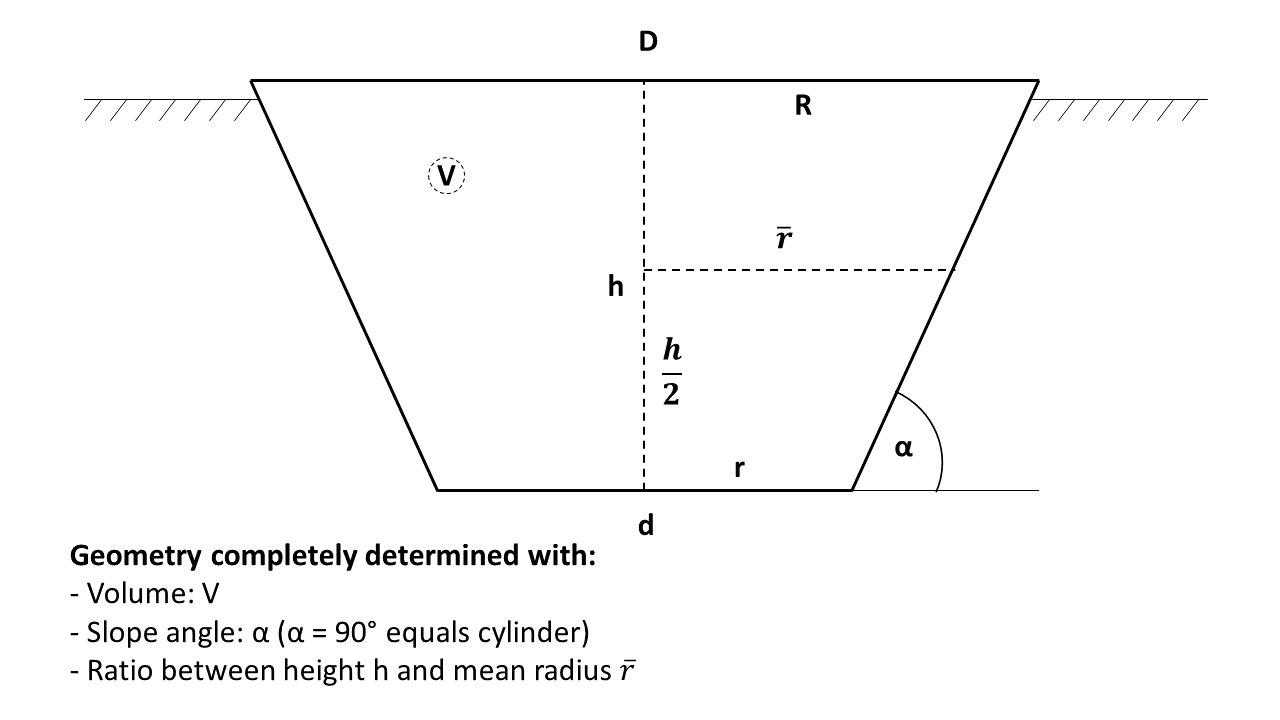Figure and method of generalized geometry definition based on [Steinacker2022]³¹.

Ratio between height and mean radius of the STES: $$hr_{STES} = \frac{h_{STES}}{\bar{r}_{STES}} = \frac{h_{STES}}{\frac{R_{STES}+r_{STES}}{2}}$$

Upper radius of the STES in dependence of the Volume and $hr_{STES}$: $$R_{STES} = \sqrt[3]{ \frac{3 \ V_{STES}}{\pi \ \tan(\alpha_{STES}) \ \left( 1 - \beta^3 \right) } } \quad \mathrm{with} \quad \beta = \frac{2 \ \tan(\alpha_{STES}) - hr_{STES}}{2 \ \tan(\alpha_{STES})+hr_{STES}}$$ Lower radius of the STES in dependence of the upper radius $R_{STES}$: $$r_{STES} = R_{STES} \ \beta$$

Slope angle has to be in the range of $$180° - \arctan{\left(\frac{hr_{STES}}{2} \right)} \geq \alpha_{STES} \geq \arctan{\left(\frac{hr_{STES}}{2} \right)}$$ to ensure the shape of a cylinder, a cone or a truncated cone. Analogously, the ratio between the height and the mean radius of the STES $hr_{LZWSP}$ has to be smaller as $$hr_{LZWSP} \leq 2 \ \tan(\alpha_{LZWSP}) \mathrm{\quad with \quad} 0 ° < \alpha_{LZWSP} < 90 °$$

The height of the STES can be calculated as $$h_{STES} = hr_{STES} \ \frac{R_{STES}+r_{STES}}{2}$$ resulting with the number of layers $n_l$ into the thickness of each layer $$\Delta z_{l} = \frac{h_{STES}}{n_l} = \text{constant for all layers}$$

Lateral surface of each layer with height $h_l$, upper radius $R_l$ and lower radius $r_l$ of each layer: $$M_{STES,l} = (R_l + r_l) \ \pi \ \sqrt{(R_l - r_l)^2 + h_l^2}$$

Volume of each layer: $$V_{STES,l} = \frac{h_l}{3} \pi \ (R_l^2 + R_l \ r_l \ + r_l^2)$$

Thermal model for stratified storage

General energy balance in every timestep $t$: $$Q_{STES,t} = Q_{STES,t-1} + (\dot{Q}_{STES,load} - \dot{Q}_{STES,unload} - \dot{Q}_{STES,loss,amb}) \ \Delta t$$

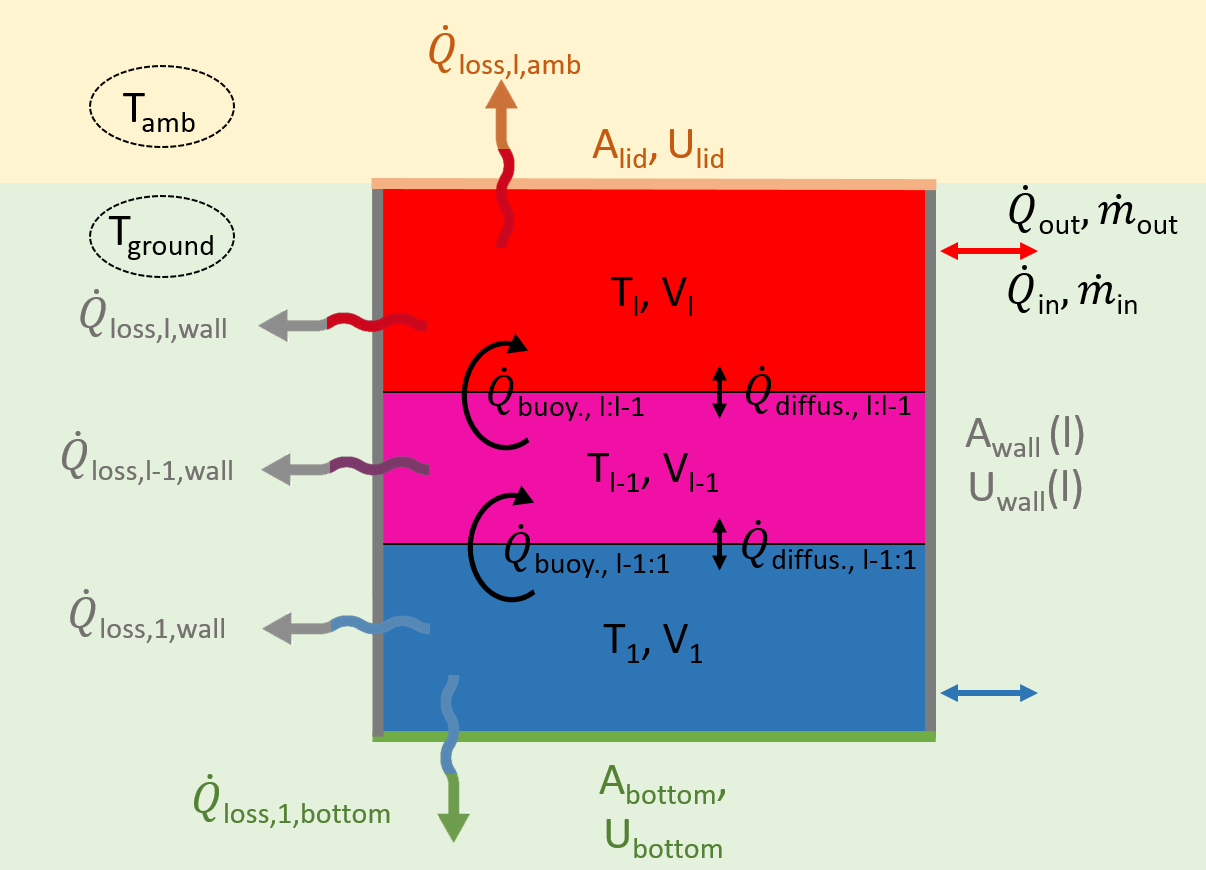Figure adapted from [Steinacker2022]³¹.

Stratified storage model based on [Lago2019]³⁰ and modified to account for cones according to [Steinacker2022]³¹ and for half-buried storages.

Three different energy or exergy loss mechanisms are taken into account as shown in the figure above:

• Energy losses to the environment through the outer walls (bottom, walls and lid) of each storage layer ($\dot{Q}_{STES,loss}$), characterized by the heat transfer coefficient of the outer surfaces $U_{STES,bottom/wall/lid}$
• Exergy losses due to diffusion processes between the storage layers $\dot{Q}_{STES,diffus.}$, specified by the diffusion coefficient $\xi_{STES}$
• Exergy losses due to convection (buoyancy) between the storage layers $\dot{Q}_{STES,buoy.}$.

The temperature $T_l$ in layer $l$ with height $\Delta z_l$ is given by the partial differential equation $$\frac{\delta T_{STES,l} }{\delta t} = \underbrace{\xi_{STES} \frac{\delta^2 T_{STES,l}}{\delta z^2}}_{\text{diffusion}} + \underbrace{\frac{M_{STES,l} \ U_{STES,l}}{\rho_{STES} \ c_{p,STES} \ V_{STES,l}} \left(T_{STES,amb,l} - T_{STES,l}\right)}_{\text{energy losses to ambient}} + \ \cdot \cdot \cdot \\ \ \\ \ \underbrace{\frac{\dot m_{STES} (T_{STES,l,in}-T_{STES,l})}{\rho_{STES} \ V_{STES,l}}}_{\text{direct (un-)loading}}$$

The ambient temperature of each layer $T_{amb,l}$ can be either the ambient air temperature $T_{amb,air}$ in the specific timestep or the ground temperature $T_{ground}$ depending on the considered layer $l$ and the number of layer buried under the ground surface.

Using the explicit Euler method for integration, the previous equation leads to the temperature in every timestep $t$ and layer $l$ with respect to the temperatures in the timestep before and the layers around (without the index $_{STES}$ for better overview) $$\begin{aligned} &T_{t+1,l} = T_{t,l} + \left( \xi_{STES} \frac{T_{t,l+1} + T_{t,l-1} - 2 T_{t,l}}{\Delta z^2_{l,vol}} + \sigma_l (T_{amb,l} - T_{t,l}) + \phi_l \dot{m}_{t,l} \left(T_{t,l,in} - T_{t,l} \right) \right) \Delta t \\ % & \text{with the volume-related layer height} \\ &\Delta z_{l,vol} = \Delta z_l \ \sqrt{\frac{n_l \ V_{STES,l}}{V_{STES}} } \ \ \text{(because \(\Delta z_l = const.\), but \(V_{STES,l} \neq const.\)),} \\[5pt] % & \text{the coefficient of heat losses to the environment} \\ &\sigma_l = \begin{cases} \frac{A_{STES,lid} \ U_{STES,lid} + M_{STES,l} \ U_{STES,l}}{c_{p,STES} \ \rho_{STES} \ V_{LZSWP,l}} &\text{for l = lid layer} \\[5pt] \frac{A_{STES,bottom} \ U_{STES,bottom} + M_{STES,l} \ U_{STES,l}}{c_{p,STES} \ \rho_{STES} \ V_{LZSWP,l}} &\text{for l = bottom layer} \\[5pt] \frac{M_{STES,l} \ U_{STES,l}}{c_{p,STES} \ \rho_{STES} \ V_{LZSWP,l}} &\text{for l = sandwich layers} \end{cases} \\ % &\text{and the coefficient for direct loading and unloading} \\ &\phi_l = \frac{1 }{\rho_{STES} \ V_{STES,l}} \ % \end{aligned}$$

As the coefficients mentioned above are constant within the simulation time, they can be precomputed for computational efficiency.

To illustrate the principle of the implemented model, the following figure shows the mass flow into and out of the STES as well as exemplary for one transition between two layers the mass flow between the layers within the model. The corresponding temperatures are the temperatures of the source (input flow or layer temperature of the previous layer). As a convention, the lowermost layer is labeled with the number 1. The inflow and outflow is always in the top and bottom layers. For correct results, the integrated mass flow within one timestep has to be smaller than the volume of the smallest layer element of the storage (ToDo: Maybe fix this issue in ReSiE?)

To account for buoyancy effects, a check is made in each timestep to determine whether the temperature gradient in the reservoir corresponds to the physically logical state, meaning that the temperatures in the upper layers are higher than in the lower storage layers. If, however, an inverse temperature gradient is present, a mixing process is performed in each timestep for all layers, beginning with $l=2$: $$T_l = T_l + \theta_l \ \text{max} (0, T_{l-1} - T_l) \text{ for } l > 1 \text{ and }\\ T_{l-1} = T_{l-1} - (1-\theta_l) \ \text{max} (0, T_{l-1} - T_l) \text{ for } l > 1$$ using the volume-ratio of each layer $\theta_l$ with respect to the surrounding layers, inspired by [Lago2019]³⁰: $$\theta_{l} = \frac{V_{STES,l-1}}{V_{STES,l} + V_{STES,l-1}} \in [0,1] \text{ for } l > 1.$$

This method was extensively tested in [Steinacker2022]³¹ and compared to calculations performed with TRNSYS Type 142 with high agreement. Is was shown that an optimal number of layers for this model is 25, considering computational efficiency and quality of the results.

Inputs and Outputs of the STES:

Symbol	Description	Unit
$\dot{Q}_{STES,load}$	thermal power input in the STES	[W]
$\dot{Q}_{STES,unload}$	thermal power output of the STES	[W]
$\dot{m}_{STES,load}$	current mass flow rate into the STES	[kg/h]
$\dot{m}_{STES,unload}$	current mass flow rate out of the STES	[kg/h]
$T_{STES,load,hot}$	temperature of input mass flow while loading the STES	[°C]
$T_{STES,load,cold}$	temperature of output mass flow while loading the STES	[°C]
$T_{STES,unload,hot}$	temperature of input mass flow while unloading the STES	[°C]
$T_{STES,unload,cold}$	temperature of output mass flow while unloading the STES	[°C]

Parameter of the STES:

Symbol	Description	Unit
$Q_{STES,rated}$	rated thermal energy capacity of the STES	[MWh]
$x_{STES,start}$	thermal energy contend of the STES at the beginning of the simulation in relation to $Q_{STES,rated}$	[%]
$T_{STES,hot}$	rated upper temperature of the STES	[°C]
$T_{STES,cold}$	rated lower temperature of the STES	[°C]
$c_{STES,max,load}$	maximum charging rate (C-rate) of STES	[1/h]
$c_{STES,max,unload}$	maximum discharging rate (C-rate) of STES	[1/h]
$V_{STES}$	volume of the STES	[m$^3$]
$\alpha_{STES,slope}$	slope angle of the wall of the STES with respect to the horizon	[°]
$hr_{STES}$	ratio between height and mean radius of the STES	[-]
$\rho_{STES}$	density of the heat carrier medium in the STES	[kg/m$^3$]
$cp_{STES}$	specific heat capacity of the heat carrier medium in the STES	[kJ/(kg K)]
$\xi_{STES}$	coefficient of diffusion of the heat carrier medium in the STES into itself	[m$^2$/s]
$U_{STES,lid}$	heat transfer coefficient of the STES' lid	[W/m$^2$ K]
$U_{STES,wall}$	heat transfer coefficient of the STES' wall	[W/m$^2$ K]
$U_{STES,bottom}$	heat transfer coefficient of the STES' bottom	[W/m$^2$ K]
$n_{STES,layers,total}$	number of thermal layer in the STES for the simulation	[pcs.]
$n_{STES,layers,above \ ground}$	number of thermal layer of the STES above the ground surface	[pcs.]
$\boldsymbol{T}_{STES,ground}$	timeseries or constant of ground temperature	[°C]
$\boldsymbol{T}_{STES,amb}$	timeseries of ambient temperature	[°C]

State variables of the STES:

Symbol	Description	Unit
${Q}_{STES}$	current amount of thermal energy stored in the STES	[MWh]
$x_{STES}$	current charging state of the STES	[%]
$\boldsymbol{T}_{STES}$	vector of current temperatures in every layer of the STES	[°C]

Borehole thermal energy storage (BTES)

Borehole thermal energy storages are not implemented yet (ToDo).

Aquifer thermal energy storage (ATES)

Aquifer thermal energy storages are not implemented yet (ToDo).

Ice storage (IS)

Ice storages are not implemented yet (ToDo).

Hydrogen fuel cell (FC)

Hydrogen fuel cells are not implemented yet (ToDo).

Photovoltaik (PV)

For the calculation of the electrical power output of photovoltaic systems, a separate simulation tool was developed and integrated into ReSiE. It is based on the Python extension pvlib³³ and uses the model chain approach described in the pvlib documentation. Technical data of specific PV modules and DC-AC inverters are taken from the SAM model³² and integrated into pvlib.

Inputs can include orientation, tilt, ambient albedo, type of installation (e.g. roof-added, free-standing), as well as module interconnection and specific PV modules and inverters chosen from the library. Additional losses, such as ohmic losses in cables or losses due to soiling, can be taken into account. A weather input dataset is required that includes direct normal, global horizontal and diffuse horizontal irradiance as well as ambient (dry bulb) temperature, humidity and wind speed.

Wind power (WP)

windpowerlib (ToDo)

Achtung: Winddaten von EPW nicht geeignet!

Battery (BA)

Energy balance of battery in every timestep: $$E_{BA,t+1} = E_{BA,t} + \Delta t \ ( \eta_{BA,charge} \ P_{el,BA,in} - \ \frac{P_{el,BA,out}}{\eta_{BA,discharge}} - P_{el,BA,loss,self})$$

Self-Discharge losses of battery: $$P_{el,BA,loss,self} = r_{BA,self \ discharge} \ \frac{1 \ h}{\Delta t} \ E_{BA,t}$$

Charging losses of battery: $$P_{el,BA,loss,charge} = (1 - \eta_{BA,charge}) \ P_{el,BA,in}$$

Discharging losses of battery: $$P_{el,BA,loss,discharge} = \frac{1 - \eta_{BA,discharge}}{\eta_{BA,discharge}} \ P_{el,BA,out}$$

Current maximum capacity of the battery: $$E_{BA,max,current} = E_{BA,rated} \ (1-r_{BA,CapReduction}) ^{ n_{cycles \ performed}}$$ $$\text{with} \ n_{cycles \ performed} = \frac{\int_{start}^{current} P_{el,BA,in} dt}{E_{BA,rated}}$$

Limits of electrical power in- and output (limit to current energy content and maximum c-rate of battery): $$\frac{E_{BA,max,current} - E_{BA}}{\Delta t \ \ \eta_{BA,charge} } \stackrel{!}{\geq} P_{el,BA,in} \stackrel{!}{\leq} c_{BA,max,charge} \ E_{BA,max,current}$$ $$\eta_{BA,discharge} \ \frac{E_{BA}}{\Delta t} \stackrel{!}{\geq} P_{el,BA,out} \stackrel{!}{\leq} c_{BA,max,discharge} \ E_{BA,max,current}$$

Relation between current charging state in percent and in energy content: $$E_{BA} = E_{BA,max,current} \ x_{BA}$$

Inputs and Outputs of the BA:

Symbol	Description	Unit
$P_{el,BA,in}$	electrical power input in the BA	[W]
$P_{el,BA,out}$	electrical power output of the BA	[W]
$P_{el,BA,loss,self}$	electrical power losses of the BA due to self-discharging	[W]
$P_{el,BA,loss,charge}$	electrical power losses of the BA while charging	[W]
$P_{el,BA,loss,discharge}$	electrical power losses of the BA while discharging	[W]

Parameter of the BA:

Symbol	Description	Unit
$\eta_{BA,charge}$	charging efficiency of battery	[-]
$\eta_{BA,discharge}$	discharging efficiency of battery	[-]
$r_{BA,self \ discharge}$	self-discharge rate of battery (% losses per hour regarding current energy content)	[1/h]
$c_{BA,max,charge}$	maximum charging rate (C-rate) of battery	[1/h]
$c_{BA,max,discharge}$	maximum discharging rate (C-rate) of battery	[1/h]
${E}_{BA,rated}$	rated electrical energy capacity of the battery	[MWh]
$r_{BA,CapReduction}$	percentage of the reduction of the current battery capacity due to one full charge cycle	[%/cycle]
${E}_{BA,start}$	electrical energy contend of the battery at the beginning of the simulation	[MWh]

State variables of the BA:

Symbol	Description	Unit
${E}_{BA}$	current amount of energy stored in the battery	[MWh]
${E}_{BA,max,current}$	current maximum capacity of the battery depending on the number of charging cycles already performed	[MWh]
$x_{BA}$	current charging state of the battery	[%]

Hydrogen compressor (HC)

ToDo

• In Tabelle Parameter nur Parameter, die auch eingegeben werden, alle anderen im Text einführen
• check for consistency: part-load, timestep, start-up, shut-down

References