Validation of energy system components

In this section, the validation of single components of ReSiE is described. A validation of further detailed components and of whole energy systems will follow.

Geothermal probe

The implementation of the model of the geothermal probes, as described in the corresponding chapter, has been validated against measurement data and the commercial, widely used software Energy Earth Designer (EED) that uses a similar approach with g-functions as the model in ReSiE does. As measurement data, the project "GEW" in Gelsenkirchen, Germany was used. The monitoring project is described in detail in the publication Bockelmann2021¹. Here, a probe field with 36 probes is investigated, including regeneration of the geothermal probe field using a reversible heat pump. For the validation presented here, the energies into and out of the probe field of the year 2014 were taken as inputs in EED and ReSiE, and the resulting average fluid temperature within the probe field was compared.

The 36 probes of the irregular shaped probe field were approximated using a rectangle shape with 3 x 12 probes with a distance of 8 m each in ReSiE, as there are no double-row L-configurations available as they are in EED, which would fit best to the original shape of the probe field. The g-function for this probe field was taken from the open source library by Spitler and Cook². The thermal properties of the soil are known from a thermal response test at the site.

The results showed a high sensibility to the soil parameters and the thermal borehole resistance (or the parameters required to calculate it). The different probe field configuration in EED, a double L-configuration, compared to a rectangle in ReSiE, has almost no effect on the results. The undisturbed ground temperature and also the temperature spread, that is assumed for the energy loading and unloading of the probe field, are also quite sensitive to the resulting average fluid temperature in the detailed model in ReSiE, as this directly affects the velocity of the fluid in the pipes and therefore the thermal resistance of the borehole. In the case study investigated, the power of the regeneration was much higher than the power of heat extraction, and therefore the temperature spread of loading had to be adjusted to meet the reality. The maximal output and input power was set very high to not limit the external energy sink and source into and out of the probe field. The thermal borehole resistance was calculated with the detailed model in ReSiE, but the simplified model with a constant thermal borehole resistance of $0.1~W/(Km)$ shows also very good results in the comparison given the highly reduced amount of required input parameters.

For a better overview, the daily averaged mean temperature within the probe field is compared between ReSiE (both simplified and detailed model), EED and the measurement data in the figure below. In the following table, the mean and the maximum absolute temperature differences are given, calculated for a timestep of one hour. Below, a line plot is comparing the daily averaged temperature of all four variants for an exemplary week.

compared variants	mean abs. temp. diff. [K]	max. abs. temp. diff. [K]
ReSiE (detailed) vs. Measurement	0.47	6.24
ReSiE (detailed) vs. EED	0.22	1.41
ReSiE (simplified) vs. Measurement	0.44	6.24
ReSiE (simplified) vs. EED	0.40	1.97

Here, one week of the figure above is plotted with a higher temporal resolution of one hour, showing the high level of agreement between the results of ReSiE, EED and the measurement data:

Below, a simulation of 25 years between ReSiE and EED is compared. The energy input and output profiles used in the validation described above are repeated for all 25 years. As the energy for regeneration is nearly the same as for energy extraction from the probe field, there is not much of a change in the average probe field temperature within the 25 years simulated. The comparison shows slight differences in the long term behaviour of the probe field of EED compared to ReSiE. This deviation was not further investigated so far but the differences are assumed to be neglectable. They do not originate from the different probe field layout, as the use of a rectangle probe field in EED has nearly no effect on the results, even after 25 years of simulation. The mean absolute temperature difference over 25 years between EED and ReSiE detailed (one hour resolution) is $0.35~K$ and the maximum deviation is $1.68~K$.

The input parameter of the simulation above is given in the following table. The highlighted values differ between the models:

Parameter and unit	Value ReSiE	Value EED	Value reality
probe field geometry	3x12 rectangle	"10x10 L2-conf."	36 irregular L-shape
borehole spacing [m]	8	8	irregular, 8 m in average
probe depth [m]	150	150	150
probe type [-]	double-U	double-U	double-U
borehole diameter [m]	0.16	0.16	0.16
shank spacing [m]	0.1	0.1	?
grout heat conductivity [W/(Km)]	2.0	2.0	?
effective thermal resistance [(Km)/W]	0.1 / calculated	calculated	?
soil undisturbed ground temperature [°C]	13	13	12
soil heat conductivity [W/(Km)]	1.6	1.6	1.6 (from thermal response test)
soil density [kg/m³]	1800	1800	? (clay and silt)
soil specific heat capacity [J/(kgK)]	2400	2400	2400
ground heat capacity [MJ/(m³/K)]	-	4.32	?
pipe diameter outer [m]	0.032	0.032	0.0320
pipe diameter inner [m]	0.0262	0.0262	0.0262
pipe heat conductivity [W/(Km)]	0.42	0.42	?
fluid specific heat capacity [J/(kgK)]	3795	3795	3795
fluid density [kg/m³]	1052	1052	1052
fluid kinematic viscosity [m²/s]	3.9e-6	-	?
fluid dynamic viscosity [Kg/(ms)]	-	4.103e-3	?
fluid heat conductivity [W/(Km)]	0.48	0.48	0.48
fluid prandtl number [-]	31.3	?	31.3
borehole wall start temperature [°C]	13	13	?
unloading temperature spread [K]	1.5	-	0.62 in average
loading temperature spread [K]	4.0	-	1.22 in average

The profile of the input (regeneration) and output (heating) energy of the probe field (Wh in 15 min resolution) as well as the input and result files of EED and ReSiE (average fluid temperature, hourly resolution, in °C) can be downloaded here.

Also, a simulation performed with different time steps has been compared, from 15 minutes to 4 hours, showing only slight and expected differences in the average fluid temperature, caused by the different time resolution.

Geothermal collector

The implemented model of the geothermal collector is based on the TRNSYS Type 710³. Therefore, a validation of the implementation was done using the same TRNSYS Type for different simulations, comparing the mean fluid temperature of the collector. DELPHIN 6.1.6 was used to perform additional analogous simulations, which also considers the moisture content and transport within the soil. DELPHIN was originally developed as simulation program for coupled heat, moisture and mass transport in capillary-porous building materials by the University of Dresden⁴.

Also, measurement data of a geothermal collector were used to compare the behaviour of all three simulation models with reality. However, the ground properties were not reliably known and only one month of continuous data without corruptions were available, limiting the validity of the results. Additionally, ahead and during this month, a lot of rain occurred, leading to a very high moisture content in the soil.

First, the geothermal collector was simulated with all three simulations models for one year without any energy extraction to evaluate the behaviour of the finite element model without load. Here, difficulties occured in the determination of the initial conditions, especially the temperature distribution in the soil, leading to small deviations at the beginning of the simulation time. The models of ReSiE and TRNSYS show strong similarities, which is not surprising as the models are very similar. DELPHIN has slight deviations, which can be explained by the more detailed model that takes both moisture content and moisture transport into account.

compared variants	mean abs. temp. diff. [K]	max. abs. temp. diff. [K]
ReSiE vs. DELPHIN	0.74	1.91
ReSiE vs. TRNSYS	0.16	1.18

Then, a realistic energy demand profile for heating and hot water of a 2.500 m² building with 85 % living and 15 % commercial usage was used to evaluate the dynamic behaviour of the models. Especially in summer, small deviations between ReSiE and TRNSYS are visible, but an overall congruency can be observed. In short term analysis, the model in ReSiE shows stronger gradients in the change in extraction power compared to TRNSYS, which may originate from the different model of the thermal transport from fluid to the pipe-surrounding soil. Overall, all three models show acceptable differences.

compared variants	mean abs. temp. diff. [K]	max. abs. temp. diff. [K]
ReSiE vs. DELPHIN	0.92	4.87
ReSiE vs. TRNSYS	0.92	2.12

As third analysis, a constant energy demand of 55 kW was taken from the collector over the span of three years. Here, especially the freezing effects of the soil can be observed. While ReSie and TRNSYS are quite similar, with small deviations in the freezing process, likely due to a different discretization of the numerical grid, the DELPHIN model obviously does not account for the additional thermal energy in the melting and freezing process in this case. In summer, small deviations of ReSiE and TRNSYS can be observed, but they are in the range of less than one Kelvin.

compared variants	mean abs. temp. diff. [K]	max. abs. temp. diff. [K]
ReSiE vs. DELPHIN	1.23	5.09
ReSiE vs. TRNSYS	0.31	3.44

In the following, the simulation results compared to the measurement data of one month, November, are shown. For the simulations local weather data from a nearby weather station were used. Here, the initial temperature distribution and the physical properties of the soil were completely unknown, which limits the validity of the results, as some parameters had to be determined iteratively, meaning the simulation results were fitted to the measurement data. Nevertheless, after the parameter fit the dynamic behaviour of the models was shown to be in agreement with each other and with the measurement data.

compared variants	mean abs. temp. diff. [K]	max. abs. temp. diff. [K]
ReSiE vs. DELPHIN	0.62	2.34
ReSiE vs. TRNSYS	0.55	2.13
ReSiE vs. Measurements	0.37	1.76
DELPHIN vs. Measurements	0.45	1.83
TRNSYS vs. Measurements	0.49	3.42

In ReSiE the detailed model for the energy transport from fluid to soil was used, while the numerical mesh was of type "normal". All ambient data were read from a weather file. The following parameters were used for the simulations of the comparison of ReSiE, TRNSYS and DELPHIN:

Variable	Value
accuracy_mode	"normal"
phase_change_upper_boundary_temperature	-0.25 °C
phase_change_lower_boundary_temperature	-1.0 °C
number_of_pipes	47
pipe_length	93 m
pipe_spacing	1.02 m
pipe_laying_depth	2.0 m
pipe_radius_outer	0.02 m
considered_soil_depth	10.0 m
soil_specific_heat_capacity	850 J/(kgK)
soil_specific_heat_capacity_frozen	850 J/(kgK)
soil_density	1900 kg/m³
soil_heat_conductivity	2.4 W/(mK)
soil_heat_conductivity_frozen	2.9 W/(mK)
soil_specific_enthalpy_of_fusion	90000 J/K
surface_convective_heat_transfer_coefficient	14.7 W/(m² K)
surface_reflection_factor	0.25
surface_emissivity	0.9
unloading_temperature_spread	3.0 K
start_temperature_fluid_and_pipe	15.5 °C
undisturbed_ground_temperature	9.0 °C
pipe_thickness	0.0037 m
pipe_heat_conductivity	0.4 W/(mK)
fluid_specific_heat_capacity	3944 J/(kgK)
fluid_heat_conductivity	0.499 W/(mK)
fluid_density	1025 kg/m³
fluid_kinematic_viscosity	3.6e-6 m²/s
fluid_prantl_number	30

The parameters for the comparison with the measurement data were deviating as follows, due to extremely wet conditions, the beginning of the heating season and therefore warm soil, and the high volume flow through the collector:

Variable	Value
soil_specific_heat_capacity	2100 J/(kgK)
unloading_temperature_spread	0.2 K
undisturbed_ground_temperature	11.0 °C
start_temperature_fluid_and_pipe	16.0 °C

In DELPHIN, a thermal transmission from fluid to pipe of 50 W/m²K for the normal simulations and 700 W/m²K for the measurement data was used.

Solarthermal collector

To validate the model for solarthermal collector and the solar irradiance calculations, it is compared to TRNSYS as well as measurement data. In the first analysis the focus is on the direct comparison between ReSiE and TRNSYS that both use a model based on DIN EN ISO 9806:2017⁵ internally while using different approaches when it comes to the solar irradiance calculations and calculation of dynamic behaviour. The goal is to show the general viability of the implemented model. In the second chapter ReSiE and TRNSYS are compared against measurement data from a real project with weather data from the closest weather station. To goal of this part is to show how well the models of ReSiE and TRNSYS are in predicting real time performance under imperfect data availability.

Validation against TRNSYS 18

For the model validation against TRNSYS 18 a typical usage profile of the solarthermal collector is created. Flat plate collectors combined with an air source heat pump are used to supply a newly build single family house with heat for heating and hot water. A buffer tank helps to store excess heat. The control for the solarthermal collector uses a fixed flow rate as soon as heat can be delivered to the buffer tank. To focus the validation on the solarthermal collector model and ignore the effects of other components in the full system simulation, only the inputs and outputs of the collector are used in the following analysis. In TRNSYS Type 1286 is used to simulate the collector and Type 15-10 to calculate the solar irradiance in the collector plane. In ReSiE the system is modelled by using only the solarthermal collector and an infinite heat demand. The flow rate and input temperature profiles are given to the collector and the output temperature and generated heat are compared to TRNSYS. Additionally the calculated irradiances in the collector plane are compared to show differences that could influence the results outside of the collector model.

The used parameters are shown in this table:

Variable	Value
collector_gross_area	16.38 m²
tilt_angle	30 °
azimuth_angle	0 °
eta_0_b	0.734
K_b_t_array	[1.00, 1.00, 0.99, 0.98, 0.96, 0.89, 0.71, 0.36, 0.00]
K_b_l_array	[1.00, 1.00, 0.99, 0.98, 0.96, 0.89, 0.71, 0.36, 0.00]
K_d	0.97
a_params	[3.96, 0.011, 0.000, 0.00, 11450, 0.000, 0.00, 0.0]
vol_heat_capacity	3.903255e6 J/(m³K)
wind_speed_reduction	1.0
ground_reflectance	0.4

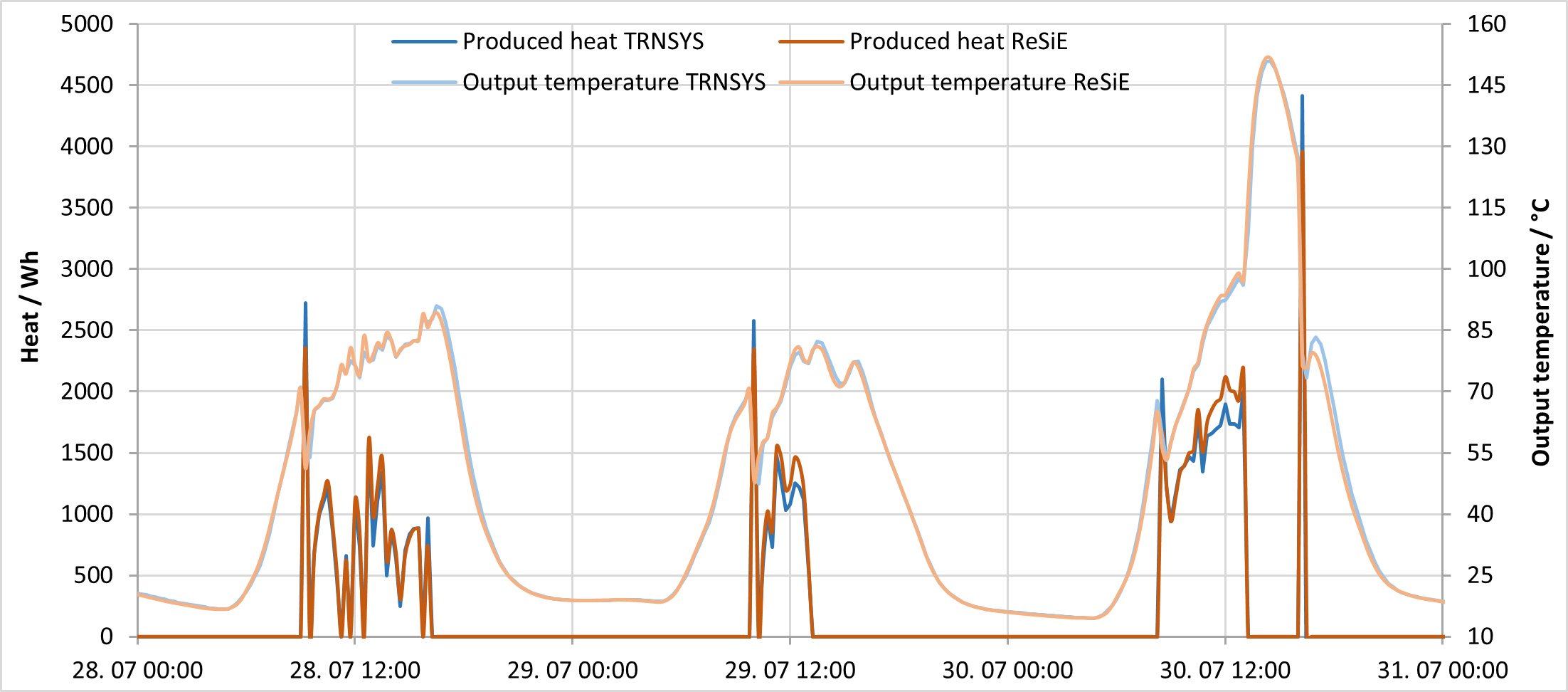
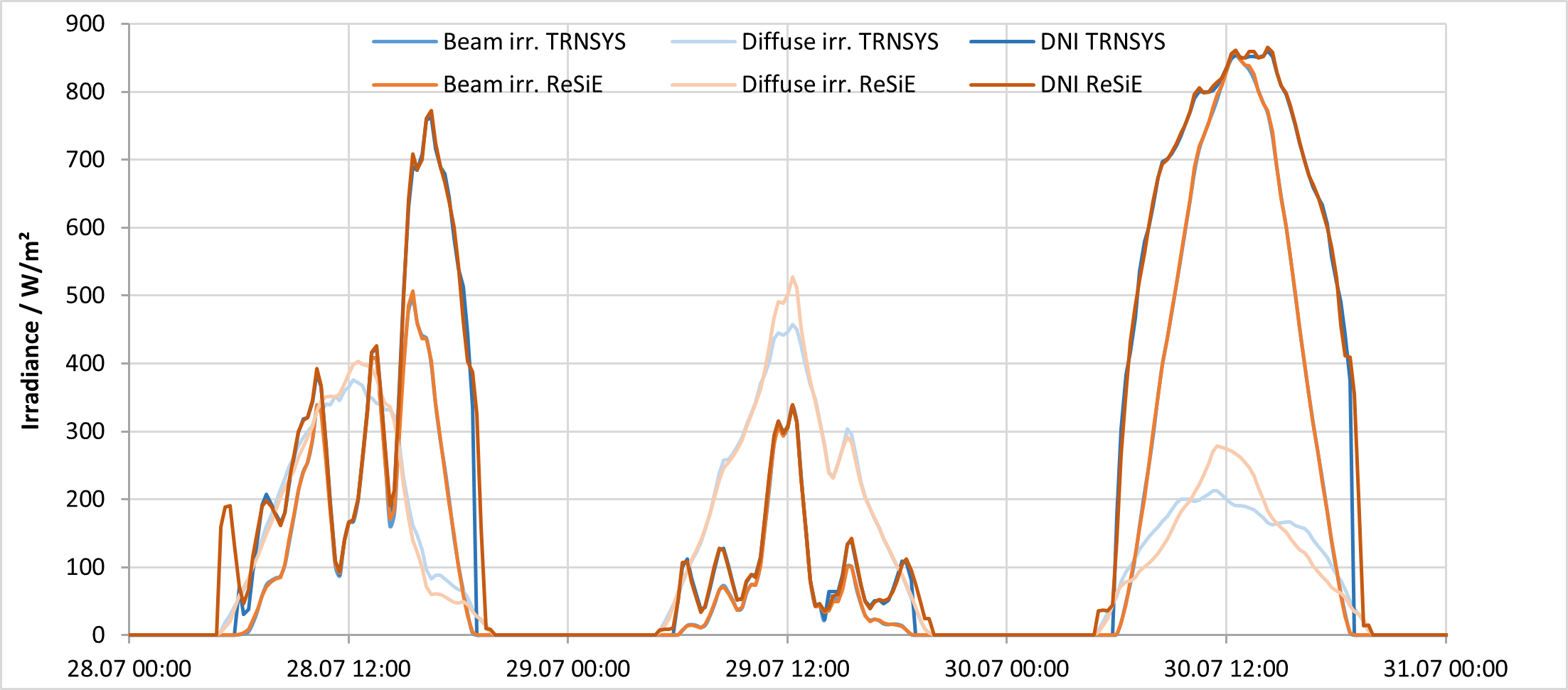
In comparison to TRNSYS ReSiE shows -3.8 % difference in produced heat. This can be largely attributed to the different model used for the diffuse irradiance which results in -6.2 % reduced diffuse irradiance and -2.9 % total irradiance in the collector plane. When the ReSiE model is run with given irradiances from TRNSYS the difference in produced heat is reduced to 0.8 %. If we take a more detailed look at the model behaviour in an example of three summer days in the following figures we notice two main effects. The first one is, that at the start of the collector operation (first time step with flow rate >0) the ReSiE model shows a less strong dynamic reaction. The produced heat in the first time step is usually lower than TRNSYS but dropping less in the next time step. This effect might be connected to TRNSYS using subtimesteps for simulation and modelling a collector array with multiple collectors in series. The second effect is that the output temperature of the ReSiE model is higher during the middle of the day (e.g. at 30.07 12:00), which can be attributed to the difference in the diffuse irradiance model, which is visible in the second figure.

In the next table are the mean and the maximum absolute temperature differences given for a few different cases. - w/o irradiance means that the irradiance values of TRNSYS is used instead of it's own irradiance calculation. - w/o operation start means that the first timestep after the start of operation is ignored. - in operation means that all values are ignored if the flow rate is 0.

compared variants	mean abs. temp. diff. [K]	max. abs. temp. diff. [K]
ReSiE vs. TRNSYS	0.68	15.7
ReSiE vs. TRNSYS in operation	0.76	4.66
ReSiE vs. TRNSYS w/o operation start	0.63	3.83
ReSiE w/o irradiance vs. TRNSYS	0.37	10.9
ReSiE w/o irradiance vs. TRNSYS in operation	0.30	3.73
ReSiE w/o irradiance vs. TRNSYS w/o operation start	0.23	3.73

Validation against measurement data

In the second step the model is validated against measurement data. For this case a multifamily house is with a heat pump and solarthermal absorbers on the roof is chosen. The measurement data covers outside air temperature, temperature at the collector output, flow rate and temperature to the collector. The flow rate and temperature to the collector are measured in the building basement, while the output temperature is measured at the collector. The wind speed and irradiance values are taken from the nearest weather station of the DWD (Deutscher Wetterdienst). The parameters in the data sheet of the collector are given for the old standard DIN EN ISO 9806:2013 and are converted to DIN EN ISO 9806:2017 using ⁶. The input parameters for ReSiE are given in the following table.

Variable	Value
collector_gross_area	430 m²
tilt_angle	5 °
azimuth_angle	0 °
eta_0_b	0.5664
K_b_t_array	[1.00, 1.00, 1.00, 1.00, 1.00, 0.89, 0.71, 0.36, 0.00]
K_b_l_array	[1.00, 1.00, 1.00, 1.00, 1.00, 0.89, 0.71, 0.36, 0.00]
K_d	0.96
a_params	[43.41, 0, 3.59, 0.47855, 3906, 0.04633, 0.03938, 0]
vol_heat_capacity	3.921470e6 J/(m³K)
wind_speed_reduction	1.0
ground_reflectance	0.4

The difference in produced heat between measurements and ReSiE is +8.5 % for ReSiE. This is a very good result, if we take into consideration the irradiance and wind speed data is wasn't available as locally measured values but only from the closest weather station. It brings a high uncertainty considering local effects on wind speed through surrounding buildings and on irradiance through clouds. Another effect to take into consideration is the difference in measuring the output temperature at the collector and the input temperature and flow rate in the building basement. This decouples the values slightly considering the long pipes running from the basement to the roof.

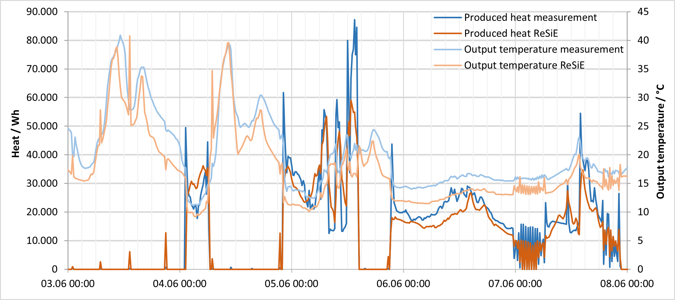
The figure below shows 5 days in the beginning of June highlighting the differences between simulation and measurement. The biggest difference can be seen when the operation is only active for one timestep for example on the 03.06 or at the beginning and end of the operation. This can be attributed to misleading measurements. The measurements are only available in 15 minute timesteps but internally the sensors create a mean value over those 15 minutes. So if the water flow is active for only 5 minutes the flow rate is reported as 1/3 over the whole timestep. The same is true for the temperature. When the water flow is active, usually fresh cold water is replacing the warmed up stale water in the pipes, which shows up as a temperature drop in the input temperature. If the water flow is active only for the last 5 minutes of a timestep the temperature is average with the higher values from the first 10 minutes, leading to a higher mean value and a wrong response from the simulation model.

The mean and maximum absolute temperature differences are given in the next table analogous to the validation against TRNSYS. As expected the differences are higher than in the synthetic comparison against TRNSYS, but still give good results during the operation of the collector.

compared variants	mean abs. temp. diff. [K]	max. abs. temp. diff. [K]
ReSiE vs. Measurement	2.83	38.3
ReSiE vs. Measurement in operation	0.87	21.4
ReSiE vs. Measurement w/o operation start	0.42	18.9

Heat pump

Due to the variations in heat pump technology and the heat sources supplying them, multiple data sets of different energy system have been included for validation of the model. A Jupyter notebook has been developed to perform the same analyses for all data sets, which is included in the documentation and can be found here. The notebook reads in the measurement data, applies manual corrections, performs data restructuring and then runs the analyses to produce charts. Some manual analysis was also done to find parameters best matching the measured energy systems, as not all required information was available. This is described in more detail for the individual data sets.

In general the workflow follows these steps:

1. Read in time series of energy values for the heat input, heat output and electricity consumed, as well as the condenser output and evaporator input temperatures.
2. Create profiles for the simulation from the measurements, including heat output and the temperatures.
3. Run the simulation with these profiles and parameters for the heat pump model informed by the modelled energy system.
4. After comparing the simulated summed energy usage with the measured values, parameters with high uncertainty are adjusted and the simulation is rerun. This is repeated until the summed values match measurements to a satisfactory degree. This is a necessarily manual process because the parameter space for optimisation is large, therefore computationally expensive, and because informed decisions by the modeler are preferable over fully automatic optimisation.
5. With the simulated time series of the determined fit, further analyses are performed.

Each case also has its own criteria for detecting anomalies, that are overwritten with manual corrections, usually as linear interpolation between preceeding and following values. The reasons for the anomalies typically include:

1. Temporary wrong reporting of meter values, where either old values or zero values are reported. This can happen due to technical malfunctions and is exceedingly difficult to avoid. As the meter electronics are very reliable and the wrong values result from the monitoring process, these values can usually be fixed from inference of the correct values following the anomalies.
2. Missing data due to technical malfunctions in the monitoring process. Depending on how much data was lost, this can be infered from following values or has to be interpolated.
3. Temporary wrong temperature data. The wrong values typically fall outside the expected temperature range of the sensor entirely and are thus easy to detect, for example a hot water temperature sensor reporting a temperature of 0 °C. It is more difficult to detect values that are presumably wrong, but still fall inside the expected range, such as an air temperature sensor reporting 0 °C during a summer day.

These manual corrections necessarily alter the results of the validation and should generally be avoided. However, the comparison with simulation results requires a continuous data set, therefore removing the anomalous data values from the data set is not possible. As each data value influences the overall result only to a small degree, a small number of corrections relative to the size of the data set does not alter the result of the validation to a large degree.

Case 1: District heating / electrolyser cooling

In the district project Klimaquartier Neue Weststadt⁷, an electrolyser plant produces hydrogen, oxygen and usable heat. While the heat output of the electrolyser stacks is utilised directly in the heating and DHW networks, a significant amount of waste heat is also produced from cooling the power electronics, gas compressors and other equipment. A water-water inverter-driven 210 kW heat pump with heat medium R513A is used to make this waste heat, with a typical temperature range from 9 to 14 °C as evaporator inlet temperature, available for the heating and DHW networks with a typical temperature range from 45 to 60 °C as condenser outlet temperature.

The measurements are from the time period from 2022-11-15 to 2025-03-31. Some corrections were required for meters temporarily reporting incorrect values and missing data, which is typical for such measurements and has a low occurence rate of 0.23 %. Of note is that measurements of the entirety of the day of 2023-11-23 are missing, which have been corrected as constant usage to linearly interpolate between the preceeding and following known meter values. Because the simulation does not support leap days, the day of 2024-02-29 has been removed prior to creating the profiles used in the simulation.

	Electricity [MWh]	Heat input [MWh]	Heat output [MWh]	Losses [MWh]
Raw measurements	188.86	321.59	527.63	-
Without leap day	188.56	321.04	526.74	-
Adjusted heat input	188.56	338.18	526.74	-
Simulated	192.08	359.46	526.72	24.820
Difference	+1.87 %	+6.29 %	-0.004 %	-

	Electricity	Heat input
CV(RMSE) 15 min	16.084	188.57
NMBE 15 min	1.8637 %	11.959 %
CV(RMSE) 60 min	0.70621	1.2587
NMBE 60 min	1.8709 %	11.967 %

The first part of the table above show the values of inputs and outputs summed up over the entire time period. The second part lists the coefficient of variation (CV) of the root mean square error (RMSE) and the normalized mean bias error (NMBE) for both electricity and heat input in both the original and aggregated timestep.

Of note is that in the measurements the electricity and heat inputs do not sum up to the produced heat output, with a difference of -17.14 MWh or -5.33 %. Due to losses occuring within the heat pump, it would be expected that the sum of the inputs is slightly larger than the output, but the opposite is the case here. It is generally the case that meters measuring heat transport are inherently inaccurate. Given that both the heat input and heat output meters must be assumed inaccurate, one possible explanation is that the heat input is undercounting and the heat output is overcounting. As the heat output values are used as the exact demand values for the simulation and the electricity input meter can assumed to be very accurate, the unknown margin of the energy balance equation falls entirely on the heat input. For the comparison between measurement and simulation data of the overall sums, the missing margin of 17.14 MWh has beed added to the heat input to serve as a lower bound of the unknown real value.

The COP data for the real heat pump is not known. For the simulation model data from a comparable water-water heat pump has been taken from an online tool for manufacturer data and multiplied with a scaling factor of 0.65. This scaling factor is the primary parameter adjusted by manual analysis to find a fit. Other parameters were mostly informed by available manufacturer information⁸. Of note is a constant power loss of 500 W, which was observed in the measurements during periods of no operation. The full set of parameters can be found in the file resie_input.json for this case. With the determined fit, the electricity input sum differs by +1.87 % and the heat input sum by +6.29 % compared to the adjusted heat input.

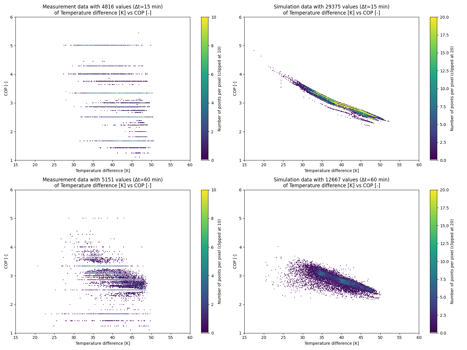
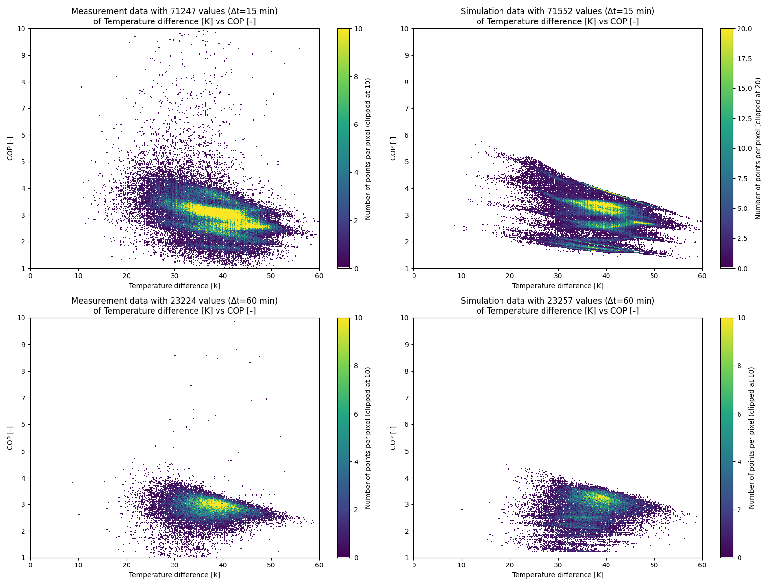
The figure above shows the values of COP over temperature difference for both measurement and simulation data, both for the original timestep of 15 minutes and for aggregated values of 60 minutes. From measurements in the original timestep, not much can be infered. In the aggregated case a clearer picture emerges, as the inverse relation between COP and temperature difference is visible in the shape and density of the point cloud. Visually comparing the aggregated measurement data with the simulation data, a reasonable match can be observed. In all four plots only data points that are active and have an absolute residual of less than 0.5 were used, where "active" refers to having both non-zero electricity input and non-zero heat output, and the absolute residual is defined as $\left| \frac{Q_{heat,in} + E_{el,in}}{Q_{heat,out}} - 1 \right|$.

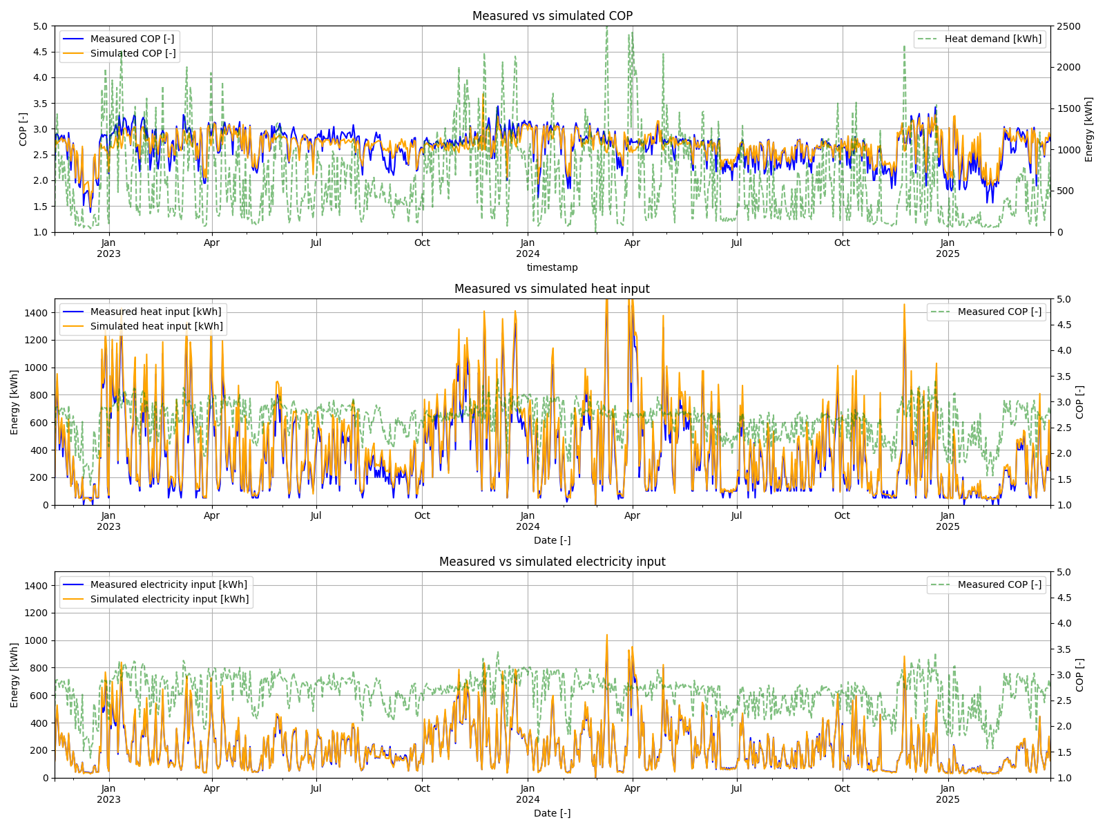
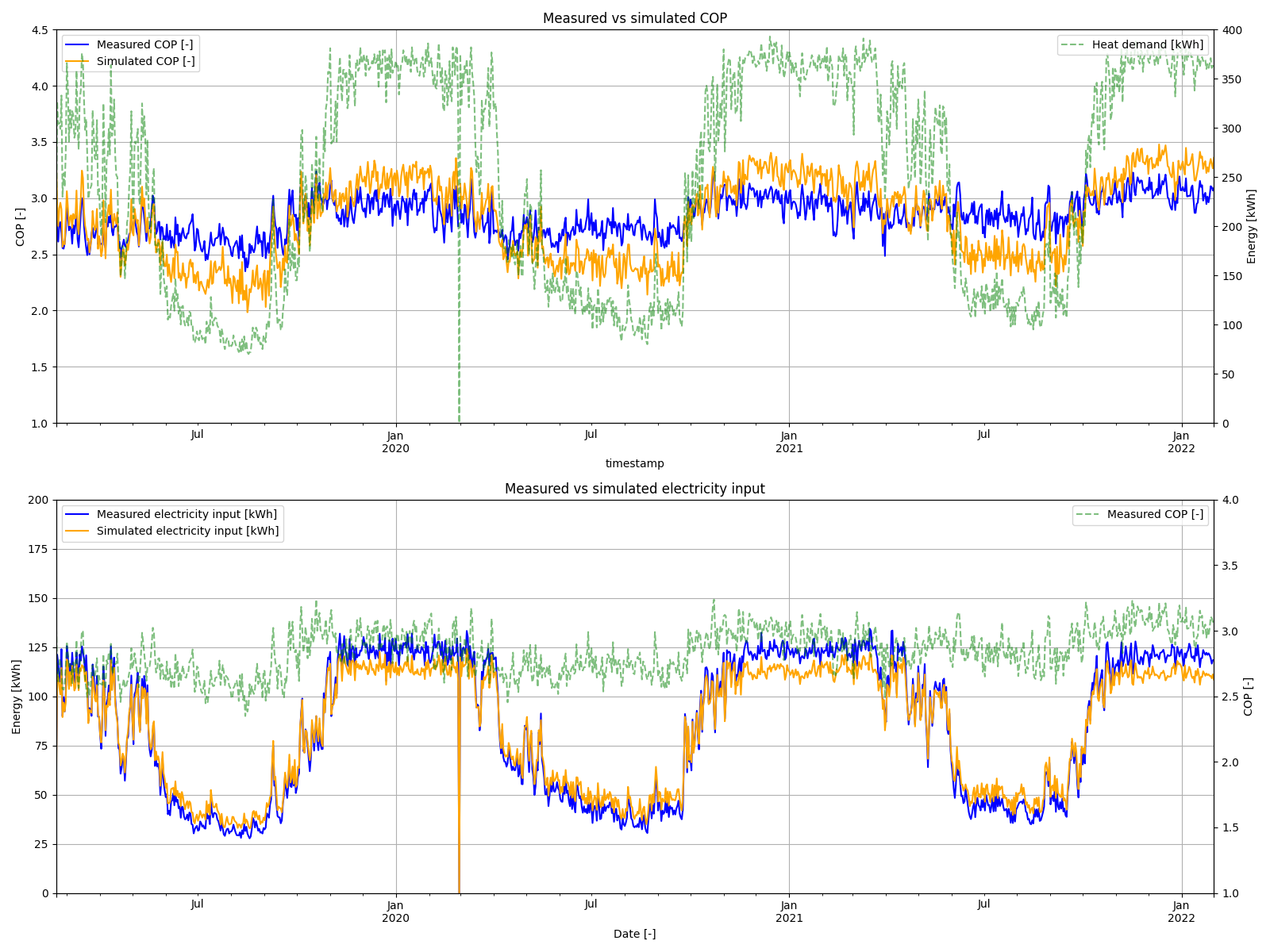
The figure above compares measurement against simulation data based on values aggregated to one day for the full period. Because the effect of meter values increasing in discrete steps compared to the actual consumption/production is lessened for aggregated values, comparing full days is expected to show a good match. Indeed, the electricity input matches closely, which can largely be attributed to it being the deciding factor in finding a parameter fit. The heat input shows the simulation data being consistently equal or higher than the measurement. Similarly the simulated COP is mostly equal or higher than the measured one, but there are some periods where the measured COP is higher, for example during July of 2023. However the measured heat input does not exceed the simulated one, which would be expected with a higher COP. It is possible that these periods contribute to the missing heat input in the overall sums.

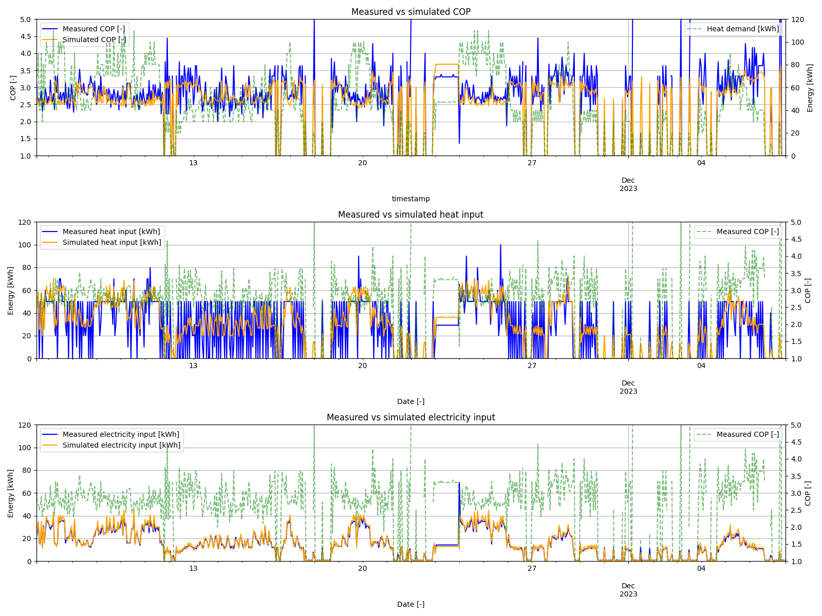
In this figure the same comparisons as above are repeated for values aggregated to one hour for a period of about one month from 2013-11-06 to 2013-12-07. This time range was chosen because it contains both periods of high and low production as well the day of 2023-11-23, which was interpolated due to missing measurements and is clearly visible in the analysis. The simulated electricity input again shows a good match with measurements. In contrast, the measured heat input displays heavy pulsing, probably due to the discrete measuring of meters. The simulated COP and heat input show a more averaged behaviour compared to the measurements.

Case 2: Multi-family home heating and DHW

In the second case measurements were taken from a multi-family home, which is supplied with domestic hot water and heat for underfloor heating by an air-sourced 26 kW on-off heat pump with heat medium R407C. No measurements for the heat energy input are available and the air temperature at the building location is also unknown, which is why the closest weather station (in Konstanz, Germany) has been used as proxy for the heat source temperature values. The measurements were preprocessed for another scientific project and require no corrections. The temperature of the mixed DHW and heating demand has a typical range from 35 °C to 60 °C. The measurements are in the time frame from 2019-02-19 to 2022-01-31. Because the simulation does not support leap days, the day of 2020-02-29 has been removed prior to creating the profiles used in the simulation.

COP field data

The COP of the heat pump is described in detail in the manufacturer's documentation ⁹ and has been inter- and extrapolated to field data with source temperatures from -20 °C to 40 °C in steps of 5 K and sink temperatures from 15 °C to 70 °C in steps of 5 K. Of note is that the vast majority of measurements fall within the range interpolated between support values, with only few values falling in the extrapolated range. These values typically occur when the heat pump starts after prolonged inactivity, when the condenser outlet has cooled off and the temperature sensor reads a cold temperature before the heat pump starts operating. The following image shows a visual representation of the interpolated field and the support values from the documentation.

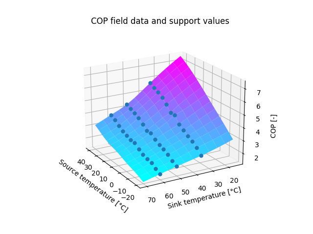
It is assumed the documentation describes the COP for the steady-state operation of the heat pump at full power at the listed temperatures, however this assumption could be wrong. It it also assumed that the COP values do not include losses due to icing of the air-liquid heat exchanger. De-icing the heat exchanger is a seperate operation mode of the heat pump during which it does not produce heat. The reduction of the COP due to icing only occurs in the model, not during real operation.

Power curve and PLF function

The documentation also describes the power curve for the thermal output power of the heat pump depending on air and demand temperatures. The influence of the demand temperature is negligible, while the source temperature is the main driver of the power curve. While the curve in the documentation shows slight non-linear behaviour, given the uncertainties it can be reasonably linearly approximated as $\dot{Q}_{th,out} = \dot{Q}_{th,max} \cdot (0.0105769 \cdot T_{source,in} + 0.576923)$. The documentation lists $\dot{Q}_{th,max}$ as 26 kW, however using this in the simulation leads to a significant fraction of unmet demand. This is likely caused by the measurements being based on meter values with a minimum accuracy of 1.0 kWh. Therefore the demand values in the measurements can differ up to 1.0 kWh from the actual demand during a timestep.

Furthermore, the temperature values and thus the output power of the heat pump vary over a timestep and are not as constant as the simulation assumes. In addition the source temperature values were taken from a weather station, not a temperature sensor at the evaporator inlet, further increasing the inaccuracy of the calculated thermal output power. To compensate for both effects $\dot{Q}_{th,max}$ has been assumed as 32 kW for the simulation. This results in an unmet demand of 740 kWh (0.28 %) over the entire timeframe.

Because the heat pump is modelled as on-off control, based on the documentation, the simulation requires choosing a PLF function to model the cycling losses incurred by the heat pump repeatedly switching on and off when the demand is less than the full available power. This is not a real technical effect and is a model assumption, therefore there is no data in the documentation to serve as a basis. An attempt to determine a PLF function from measurements was done and is described in the following. In the results section for case 2 the limitations of this approach are described.

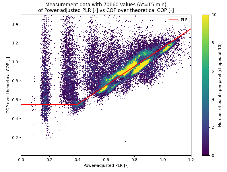
The figure above shows a scatter plot of measurement data with the power-adjusted PLR values on one axis and the ratio of the COP over theoretical COP on the other. The power-adjusted PLR has been calculated by dividing the heat demand over the maximum heat output depending on the current temperatures (affecting the maximum power). The theoretical COP is the COP calculated by the field values also depending on the current temperatures. A linear relation between the two values can be clearly observed for PLR values above 0.4 and upwards. The following PLF function has been determined as a fit and is shown as a red line in the figure:

$$PLF(\kappa) = \begin{cases} 0.55 &\text{for } \kappa \leq 0.4\ \\[5pt] \kappa + 0.15 &\text{for } \kappa \gt 0.4\ \\ \end{cases} \\ $$

The constant part for $\kappa \leq 0.4$ has been chosen for two reasons. The first is that the linear relation of the upper part is much less supported by values in this region, making an extension of the line downwards questionable. The other reason is that low values in the PLF lead to many instances of implausibly low COP values (of less than 1.0) during simulation, which indicates the linear relation being a poor fit for this region.

Results

This section discusses the results of a manually determined parameter fit. The full parameter set can be found in the file resie_input.json for case 2. Apart from the already discussed COP field, power curve and PLF function, other significant parameters include a constant 260 W electricity loss and enabling the calculation of icing losses with default parameters. Of note is that the COP field has been uniformly multiplied with a scaling factor of 1.2.

The figure above shows the values of COP over temperature difference for both measurement and simulation data, both for the original timestep of 15 minutes and for aggregated values of 60 minutes. In all four plots only active data values were used. All four plots clearly show the expected behaviour, in that a higher temperature difference leads to a lower COP. Banding effects are visible in both measurements and simulation data for the 15 minute timestep. One known cause of this is the heat demand being measured in discrete values, leading to discrete PLR values and reduction through the PLF. When the PLF is simulated as being constant, the banding in the simulation data is reduced significantly. Another possible cause is the condenser outlet temperatures being clustered around two typical ranges, one for the underfloor heating demand and one for the DHW demand, while the air temperature varies independently of that. This leads to banding when the varying air temperature values trace two different paths over the COP field data for the relatively constant output temperatures. Overall, a visual comparison of the measurements and simulation data suggests a reasonable match between them.

	Electricity [MWh]	Heat input [MWh]	Heat output [MWh]	Losses [MWh]
Raw measurements	92.49	-	266.56	-
Without leap day	92.37	-	266.24	-
Simulated	90.62	193.80	265.50	18.92
Difference	-1.89 %	-	-0.28 %	-

	Electricity	Heat output
CV(RMSE) 15 min	1.8170e-1	1.8757e-2
NMBE 15 min	-1.8938 %	-0.27117 %
CV(RMSE) 60 min	1.1390e-1	9.8077e-3
NMBE 60 min	-1.8938 %	-0.27117 %
CV(RMSE) 1 d	7.7609e-2	4.6876e-3
NMBE 1 d	-1.8938 %	-0.27117 %

The first part of the table above show the values of inputs and outputs summed up over the entire time period. The second part lists the coefficient of variation (CV) of the root mean square error (RMSE) and the normalized mean bias error (NMBE) for both electricity input and heat output in timesteps of 15 minutes, 60 minutes and one day.

For reasons mentioned in the section on the power curve there is an unmet demand of 740 kWh or 0.28 %. The electricity input is 1.89 % lower than in the measurements. This number can be reduced close to zero by fine-tuning the scaling factor for the COP field data, which was not done as it provides no additional information on the validity of the model. This becomes much clearer when the data sets are compared time-resolved, as described in the following.

The figure above shows measurements vs. simulation data for the COP and electricity input over the full time frame aggregated to daily values. For both measurements and simulation the COP values are higher in winter than in summer, which can be explained by the higher demand temperatures in summer, due to only supplying DHW, more than offsetting the gain in the COP due to higher air temperatures. The COP lines match in general behaviour of daily fluctuations, however also show the simulation data consistently being overestiamted in winter and underestimated in summer. This can be seen more clearly in the following figures, which highlight a week in August of 2021 and a week in December of 2021.

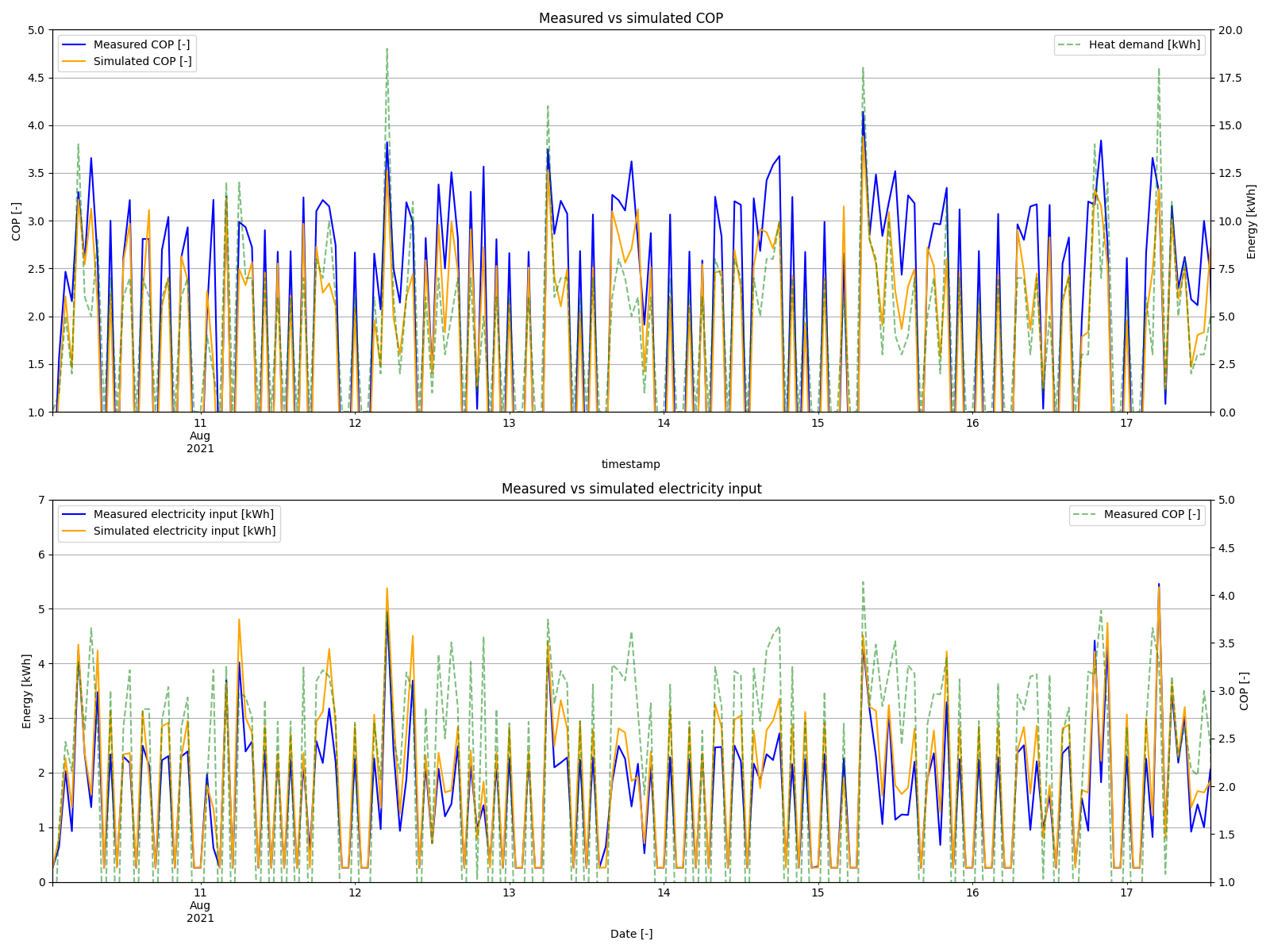
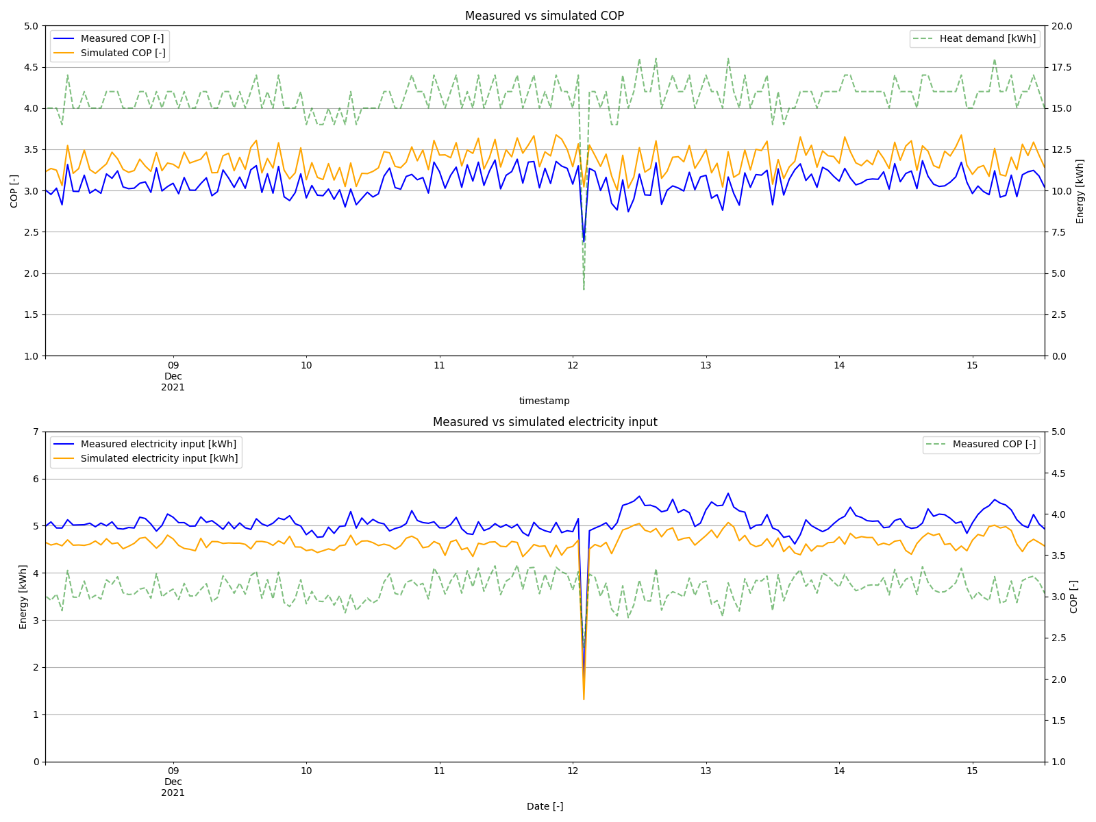
The overestimation in winter and underestimation in summer can be seen very clearly in the hourly data. In winter the heat pump is running constantly at a high PLR, while in summer it is running intermittently at a low to medium PLR. These are two scenarios where the PLF function ought to increase the accuracy of the model, yet this is not the case.

When the simulation is performed with a COP scaling factor of 1.0 and a constant PLF function of 1.0, the simulation data matches very closely in winter and is underestimating in summer. This would suggest that the real heat pump does not suffer decreased efficiency in part load operation, yet the analysis done in the corresponding section above strongly suggests that the PLF function should be modelled as such. The reasons for this discrepancy remain unclear and could be a combination of effects caused by uncertainties and inaccuracies in the measurements or it could indicate a weakness in the heat pump model concerning the PLF function. Further work in this regard is welcome.

Seasonal thermal energy storage (STES)

STES without ground-coupling against TRNSYS Type 342

Note: The validation shown here was done with the simplified ground model without FVM! For the model including ground-coupling, see the next section!

The model of the seasonal thermal energy storage in ReSiE was validated against the TRNSYS Type 342, originally developed by Bengt Eftring and Göran Hellström¹⁰ and extended by Livio Mazzarella¹¹, also known as TRNSYS Type 142 or "XST Model". The TRNSYS models includes a fully ground-coupled model of a stratified storage. Here, in ReSiE, the thermal exchange to the ground is modeled with a user-defined ground temperature (constant or profile), neglecting any thermal capacity effects of the ground. The ground-coupling is taken into account in the comparison to simulations results in the IEA ES Task 39 described below.

For the validation, a self-discharging and a loading and unloading pattern were compared between the two models for a cylindrical storage with 50,000 m^3 of storage volume with a h/r ratio of 1.13. In order to make the two models better comparable, a constant ambient air temperature of 20 °C is assumed. In ReSiE, a ground temperature of 9 °C is assumed, while in TRNSYS the ground is modeled with typical parameters. The storage has 75 cm of insolation at the lid and 50 cm on the sidewalls and bottom, with a thermal conductivity of 0.1875 W/(m*K).

First, lets compare the self-unloading of the storage installed fully above the ground during 5 years. The figures shows the temperature within the top and the bottom storage layer. The differences of the temperature within the storage, especially in the bottom layer, can be explained by the constant ground temperature in ReSiE compared to the FVM model in TRNSYS that includes the thermal capacity of the ground below the STES.

compared variants	mean abs. temp. diff. [K]	max. abs. temp. diff. [K]	abs. temp. diff. after 5 years [K]
ReSiE vs. TRNSYS top layer	1.23	1.54	1.2
ReSiE vs. TRNSYS bottom layer	2.59	6.51	0.7

The inputs in ReSiE are the following:

Variable	Value	Unit
constant_ambient_temperature	20	[°C]
volume	50000	[m^3]
hr_ratio	1.13	[-]
sidewall_angle	90	[°]
shape	"round"	[-]
rho_medium	1000	[kg/m^3]
cp_medium	4.18	[kJ/(kgK)]
diffusion_coefficient	0.143 * 10^-6	[m^2/s]
number_of_layer_total	25	[-]
number_of_layer_above_ground	25	[-]
high_temperature	90	[°C]
low_temperature	10	[°C]
thermal_transmission_lid	0.25	[W/(m^2K)]
thermal_transmission_barrel	0.375	[W/(m^2K)]
thermal_transmission_bottom	0.375	[W/(m^2K)]
constant_ground_temperature	9.0	[°C]
initial_load	1.0	[%/100]

To show the loading and unloading of the storage, an idealized pattern for loading and unloading was simulated both with ReSiE and TRNSYS. Here, a constant mass flow of 40.000 kg/h was assumed both for loading in January - April (input flow in top layer at 90 °C) and unloading in September - December (input flow in bottom layer at 10 °C). The parameter used are the same as for the self-discharging above. The resulting energy input and output in the storage as well as the temperature distribution within this year is shown below:

As seen in the figure, the energy and the temperature are quite close to each other. Only during self-discharging in summer, the differences between the models can be seen.

compared variants	mean energy diff.	max. energy diff.
ReSiE vs. TRNSYS Energy (absolute values)	18.4 kWh	71.9 kWh
ReSiE vs. TRNSYS Energy (relative to maximum)	0.50 %	1.93 %

compared variants	mean abs. temp. diff. [K]	max. abs. temp. diff. [K]
ReSiE vs. TRNSYS top layer	0.59	1.61
ReSiE vs. TRNSYS 75% layer	0.56	1.57
ReSiE vs. TRNSYS middle layer	0.52	1.49
ReSiE vs. TRNSYS 25% layer	0.54	1.43
ReSiE vs. TRNSYS bottom layer	0.50	1.57

The figure below shows the simulation results of the STES buried under ground with only 1 layer above and 24 layers below the ground surface. Here, the difference in the simulation results is clearly visible between the simplified model in ReSIE and the detailed FVM model of the TRNSYS Type 342. The model in ReSiE has been extended by a ground-coupling FVM which is validated below.

STES with ground coupling using test cases of IEA ES Task 39

The updated model of the STES was compared to the test cases provided by the International Energy Agency Energy Storage Task 39 (IEA ES Task 39)¹². The Task has delivered four test cases that can all be modelled with the STES model in ReSiE:

• TTES-1-AG: A cylindrical tank above ground.
• TTES-1-UG: A cylindrical tank fully buried below ground.
• PTES-1-C: A truncated cone fully buried below ground.
• PTES-1-P: A truncated pyramid fully buried below ground.

All test cases are described in detail in the deliverable C2a of the Task 39¹³. The four test cases were reproduced with ReSiE and compared to the results shared by the Task 39 participants. The input files of ReSiE and the corresponding profiles, the result files of the simulation and comparisons to the simulation results provided by the Task 39 are all available here for the four test cases listed above. An overview of the comparison to the simulation results of other simulation models provided by the Task 39 participants is shown below.

First, the yearly energy input, energy output und energy losses to the ambient are compared for the four test cases against some of the results of the other simulation tools shared by the Task 39. The relative percentage deviations to ReSiE are given above the bars. Note that only the fifth year of the simulation is compared here as defined in the test cases.

Also, the temperature of the output mass flow and the energy content in the STES are compared for each simulation case against the ReSiE baseline. For each comparison, paired time-step values are evaluated (with ReSiE on the x-axis and the respective simulation result on the y-axis). For the temperature comparison, the root mean square error (RMSE) and the mean bias error (MBE) are reported; for the energy-content comparison, the coefficient of variation of RMSE (CVRMSE) and the normalized mean bias error (NMBE) are reported.

• RMSE quantifies the typical magnitude of deviations (in the same unit as the variable, e.g. °C): $$\mathrm{RMSE}=\sqrt{\frac{1}{n}\sum_{i=1}^{n}\left(y_i-x_i\right)^2}$$

• MBE quantifies the systematic offset (bias) between the compared result and ReSiE (same unit as the variable). Positive values indicate overestimation relative to ReSiE: $$\mathrm{MBE}=\frac{1}{n}\sum_{i=1}^{n}\left(y_i-x_i\right)$$

• CVRMSE is RMSE normalized by the mean baseline value, reported in percent (useful for comparing across testcases/scales): $$\mathrm{CVRMSE}[\%]=100\cdot\frac{\mathrm{RMSE}}{\overline{x}}$$

• NMBE is MBE normalized by the mean baseline value, reported in percent. Positive values indicate overestimation relative to ReSiE: $$\mathrm{NMBE}[\%]=100\cdot\frac{\mathrm{MBE}}{\overline{x}}$$

Testcase TTES-1-AG:

Testcase TTES-1-UG:

Testcase PTES-1-C:

Testcase PTES-1-P:

Across all four year-long testcases, TRNSYS shows the most consistent agreement with the ReSiE baseline - temperature deviations are generally small (RMSE_T as low as 0.057 °C in TTES-1-AG and ≤ 1.28 °C elsewhere) with near-zero bias (|MBE_T| ≤ 0.20 °C), and the storage-energy agreement is similarly strong (CVRMSE_E mostly 0.11–1.51% and NMBE_E essentially zero in the best cases), whereas Matlab can match reasonably well in some cases (e.g., PTES-1-C temperature RMSE_T 1.69 °C) but is less robust across scenarios (notably TTES-1-UG with RMSE_T 3.30 °C and a more pronounced negative energy bias in PTES-1-C with NMBE_E -1.60%). The remaining tools (Comsol, Dymola, Modelica) exhibit systematically larger and/or more case-dependent discrepancies, most evident in TTES-1-AG where Comsol and Dymola show substantially higher energy scatter and underestimation (CVRMSE_E up to 5.44%, NMBE_E up to -5.15%) alongside markedly higher temperature RMSEs (about 3.2 °C).

Additionally, sensitivity analyses have been performed of different simulation time steps (15 min, 60 min, 120 min) and mesh resolutions (very_rough, rough, normal, high, very_high) to check the consistency of the ReSiE STES model. Exemplary, the losses of the STES to the ambient are shown below for different mesh resolutions:

Overall, ReSiE is fully in line with the other simulation environments for typical energy-supply-system use, i.e., it reproduces the relevant temperature and storage-energy behavior with deviations that remain within a practically acceptable range for system-level performance assessment and comparative studies.